esProc Improves Text Processing – Parse Logs with Arbitrary Number of Lines

When parsing logs into structured data, we often find that the records consist of a variable number of lines. This makes the conversion, as well as the corresponding operation, quite complicated. Equipped with various flexible functions for structured data processing, such as regular expressions, string splitting, fetching data located in a different row, and data concatenation, esProc is ideal for processing this kind of text. Following example will show you how it works.

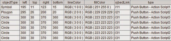
The log file reportXXX.log holds records, each of which consists of multiple lines with 14 data items (fields) and starts with the string “Object Type”. Our goal is to rearrange the log into structured data and write the result to a new text file. Some of the source data are as follows:

esProc code for doing this：

A1=file("e:\\reportXXX.log").read()

This line of code reads the logs entirely into the memory. Result is as follows:

A2=A1.array("Object Type: ").to(2,)

This line of code can be divided into two parts. The first part - A1.array("Object Type: ") – splits A1 into strings according to “Object Type”. Result is as follows: 

Except the first item, every item of data is valid. to(2,) means getting items from the second one to the last one. Result of A2 is as follows:

This line of code applies the same regular expression to each member of A2 and gets the 14 fields separated by commas. Following lists the first fields:
 

A4=file("e:\\result.txt").export@t(A3)  

This line of code writes the final result to a new file. Tab is the default separator. The use of @t option will export the field names as the file’s first row. We can see the following data in result.txt:

The regular expression used in the code above is complicated. We’ll use esProc’ built-in functions to make the operation more intuitive. For example, ObjectType field is the first line of each record, so we can separate the records from each other with the line break and then get the first line. left\top\right\bottom actually splits each record’s second line by space and get item 3, 5, 7 and 9.

The task can be handled with esProc built-in functions as follows:

In the above code, pjoin function concatenates many sets together; array function splits a string into many segments by the specified delimiter and creates a set with them, in which (~.array("\r\n") splits each record by carriage return.

In the above example, we assumed that the log file is not big and can be wholly loaded into the memory for computing. But sometimes the file is big and needs to be imported, parsed and exported in batch, which makes the code extremely difficult to write. Besides, because the number of records is variable, there is always a record in a batch of data which cannot be imported completely. This further complicates the coding.

esProc can handle the big log files with arbitrary number of lines more easily using file cursors. Following is a code sample: 

A1=file("\\reportXXX.log").cursor@s()

This line of code opens the log file in the form of a cursor. cursor function returns a cursor object according to the file object, with tab being the default separator and _1,_2…_n being the default column names. @s option means ignoring the separator and importing the file as a one-column string, with _1 being the column name. Note that this code only creates a cursor object and doesn’t import data. Data importing will be started by for statement or fetch function.

A2: for A1,10000

A2 is a loop statement, which imports a batch of data (10,000 rows) each time and sends them to the loop body. This won’t stop until the end of the log file. It can be seen that a loop body in esProc is visually represented by the indentation instead of the parentheses or identifiers like begin/end. The area of B3-B7 is A2’s loop body which processes data like this: by the carriage-return the current batch of data is restored to the text which is split into records again according to “Object Type” , and then the last, incomplete record is saved in B1, a temporary variable, and the first and the last record, both of which are useless, are deleted; and then the regular expression is parsed with each of the rest of the records, getting a two-dimensional table to be written into result.txt. Following will explain this process in detail:

B2=B1+A2.(_1).string@d("\r\n")

This line of code concatenates the temporary variable B1 with the current text. In the first-run loop, B1 is empty. But after that B1 will accept the incomplete record from the previous loop and then concatenate with the current text, thus making the incomplete record complete.

string function concatenates members of a set by the specified separator and @d function forbids surrounding members with quotation marks. Top rows in A2 are as follows:

A2.(_1) represents the set formed by field _1 in A2 :

A2.(_1).string@d("\r\n") means concatenating members of the above set into a big string, which is Object Type: Symbol Location: left: 195 top: 11 right: 123 bottom: 15 Line Color: RGB ( 1 0 0 ) Fill Color:   RGB ( 251 255 0 ) Link:l11…. 

B3=B2.array("Object Type: ")

This line of code splits the big text in B2 into strings by “Object Type”. Result of B3’s first-run loop is as follows:

Since the last string in B3 is not a complete record and cannot be computed, it will be stored in the temporary variable and concatenated with the new string created in the next loop. B4’s code will store this last string in the temporary variable B1.

B4=B1="Object Type: "+B3.m(-1)+"\r\n"

m function gets one or more members of a set in normal or reverse order. For example, m(1) gets the first one, m([1,2,3]) gets the top three and m(-1) gets the bottom one. Or B3(1) can be used to get the first one. And now we should restore the “Object Type” at the beginning of each record which has been 

deleted in the previous string splitting in A2. And the carriage return removed during fetching the text by rows from cursors will be appended.

The first member of B3 is an empty row and the last one is an incomplete row, both of them cannot be computed. We can delete them as follows:

B5=B3.to(2,B3.len()-if(A1.fetch@0(1),1,0)))

This line of code fetches the valid data from B3. If the data under processing is not the last batch, fetch rows from the second one to the second-last one and give up the first empty row and last incomplete row. But if the current batch is the last one, fetch rows from the second one and the last one which is complete and give up the first empty row only.

B3.to(m,n) function fetches rows from the mth one and the nth one in B3. B3.len() represents the number of records in B3, which is the sequence number of the last record in the current batch of data. A1.fetch(n) means fetching n rows from cursor A1 and @0 option means only peeking data but the position of cursor remaining unchanged. if function has three parameters, which are respectively boolean expression, return result when the expression is true and return result when the expression is false. When the current batch of data is not the last one, A1.fetch@0(1) is the valid records and if function will return 1; when it is the last one, value of A1.fetch@0(1) is null and if function will return 0.

B6=B5.regex(regular expression;field names list). This line of code applies the same regular expression to each member of B5 and gets the 14 fields separated by commas. Following lists the first fields:

B7=file("e:\\result.txt").export@a(B6)

This line of code appends the results of B6 to result.txt. It will append a batch of records to the file after each loop until the loop is over. We can view this example’s final result in the big file result.txt:

In the above algorithm, regular expression was used in the loop. But it has a relatively poor compilation performance, so we’d better avoid using it. In this case, we can use two esProc scripts along with pcursor function to realize the stream-style splitting and parsing.

First let’s look at the code for master routine main.dfx:

pcursor function calls a subroutine and returns a cursor consisting of one-column records. A2 parses the regular expression with each record in A1 and returns structured data. Note that the result of A2 is a cursor instead of the in-memory data. Data will be exported to the memory for computing from A2’s cursor segmentally and automatically by executing export function.

Subroutine sub.dfx is used to return the cursor, whose code is similar to the previous one. The difference is that the results need not be written to a new file, the one-column records will be returned instead, as the following code shows:

B6’s result statement can convert the result of B5 to a one-column table sequence and return it to the caller (pcursor function in main.dfx) in the form of a cursor.

With pcursor function, master routine main.dfx can fetch data from the subroutine sub.dfx by regarding it as an ordinary cursor and ignoring the process of data generation. While main.dfx needs data, pcursor function will judge if the loop in sub.dfx should continue, or if it should supply data by returning them from the buffer area. The whole process is automatic.