Method of Computing Link Relative Ratio and Year-on-year Comparison in R Language

Cross-row and -group computation often involves computing link relative ratio and year-on-year comparison.Link relative ratio refers to comparison between the current data and data of the previous period. Generally, it takes month as the time interval. For example, compare the sales amount of April with that of March, and the growth rate we get is the link relative ratio of April. Hour, day, week and quarter can also be used as the time interval.Year-on-year comparison is the comparison between the current data and data of the corresponding period of the previous year. For example, compare the sales amount of April 2014 with that of April 2013 and compute the growth rate which is April's year-on-year comparison. Data of multiple periods are usually compared to find the variation trend in practical business.

Now let's look at the method of computing link relative ratio and year-on-year comparison in R language through an example.

Case description:

Compute the link relative ratio and year-on-year comparison of each month's sales amount during a specified period of time. The data come from orders table sales, in which column Amount contains order amount and column OrderDate contains order dates. Some of the data are as follows:

Code:
sales<-read.table("E:\\ salesGroup.txt",sep="\t", header=TRUE)
filtered<-subset(sales,as.POSIXlt(OrderDate)>=as.POSIXlt('2011-01-01 00:00:00') &as.POSIXlt(OrderDate)<=as.POSIXlt('2014-08-29 00:00:00'))
filtered$y<-format(as.POSIXlt(filtered$OrderDate),'%Y')
filtered$m<-format(as.POSIXlt(filtered$OrderDate),'%m')
agged<-aggregate(filtered$Amount, filtered[,c("m","y")],sum)
agged$lrr<- c(0, (agged$x[-1]-agged$x[-length(agged$x)])/agged$x[-length(agged$x)])
result<-agged[order(agged$m),]
result$yoy<-NA
for(i in 1:nrow(result)){
if(i>1 && result[i,]$m==result[i-1,]$m){
result[i,]$yoy<-(result[i,]$x-result[i-1,]$x)/result[i-1,]$x
}
}
Code interpretation:
1. The first four lines of code are easy to understand. read.table is used to read data from the table and subset to filter data, and two format functions are used to generate year and month respectively. Note that the beginning and ending time should be output dynamically from the console using scan function; here they are simplified as fixed constants.

After computing, some of the values of database frame filtered are:

2. agged<-aggregate(filtered$Amount, filtered[,c("m","y")],sum), this line of code summates the order amount of each month of each year. Note that in the code, the month must be written before the year though data are grouped by the year and the month according to business logic. Otherwise R language will perform grouping first by the month, then by the year, which will get result inconsistent with business logic and make data viewing inconvenient.

After computing, some of the values of data frame agged are:

3. agged$lrr<- c(0, (agged$x[-1]-agged$x[-length(agged$x)])/agged$x[-length(agged$x)])，this line of code computes link relative ratio. The result will be stored in the new column Irr. Business logic is (order amount of the current month – order amount of the previous month)\order amount of the previous month.

Note: [-N] in the code represents that the Nth row of data is removed. So agged$x[-1]means the first row of data is removed andagged$x[-length(agged$x)]means the last row of data is removed. By performing certain operation between the two, link relative ratio can be obtained indirectly. But the result won’t include the link relative ratio of the first month (i.e. January 2011), so a zero should be added to the code. We can see that the code logic and the business logic share some similarities but are quite different. The code is difficult to understand.

At this point, some of the values of data frame aggedare:

4. result<-agged[order(agged$m),], this line of code sorts data by the month and the year. Since the data of the year are ordered, we just need to perform sorting by the month. result$yoy<-NA initializes a new column which will be used to store the year-on-year comparison of sales amount.

Now the value of result is:

5. The loop judgment in the last four lines of code is to compute the year-on-year comparison. Business logic: (order amount of the current month – order amount of the previous month)\order amount of the previous month. Code logic: from the second line, if the month in the current line is the same as that in the previous line, the code will compute year-on-year comparison. Detailed code is result[i,]$yoy<-(result[i,]$x-result[i-1,]$x)/result[i-1,]$x. We can see that the code written in this way is easy to understand and its logic is quite similar to the business logic.

The only weakness of this piece of code is that it cannot use the loop function of R language, which makes it a little lengthy. But compared with the difficult operation of link relative ratio, maybe a longer but simple code is better.

The final results are as follows:

Summary:

R language can compute link relative ratio and year-on-year comparison, but the operation of link relative ratio is difficult to understand and the code of year-on-year comparison is a little lengthy. The codes of both operations are not easy to learn.

The third-party solution

Python, esProc and Perl, all of which can perform structured data computation, can be used to handle this case. In the following, we'll briefly introduce esProc and Python's solutions.

esProc

esProc is good at expressing business logic freely with agile syntax. Its code is concise and easy, as shown below:

In the above code, groups function is used to group and summarize data by the year and the month. The derive functions in A4 and A6 generate link relative ratio and year-on-year comparison respectively.

As can be seen from the code,esProc also uses[-N]. Different from [-N] in R language, it doesn't represent removing the Nth row; it represents the Nth row counted from the current line. For example, [-1] is the previous line. In this way, the operation of link relative ratio can be simply expressed as (x-x[-1])/x[-1].But R language hasn't expressions for relative positions, which makes its code difficult to understand.

In the year-on-year comparison operation, esProc uses judgment function if in loop function, making it avoid the lengthy loop statement and its code simpler. While R language only has the judgment statement but hasn't the judgment function. This is the reason why its code is lengthy.

Finally, these are the computed results:

Python（Pandas）
Pandas isPython's third-party package. Its basic data type is created by imitating R's dataframe but gets improved greatly. At present, its latest version is 0.14. Its code for handling this case is as follows:
sales = pandas.read_csv('E:\\salesGroup.txt',sep='\t')
sales['OrderDate']=pandas.to_datetime(sales.OrderDate,format='%Y-%m-%d %H:%M:%S')
filtered=sales[(sales.OrderDate>='2011-01-01 00:00:00') & (sales.OrderDate<='2014-08-29 00:00:00')]
filtered['y']=filtered.OrderDate.apply(lambda x: x.year)
filtered['m']=filtered.OrderDate.apply(lambda x: x.month)
grouped=filtered.groupby(['y','m'],as_index=False)
agged=grouped.agg({'Amount':[sum]})
agged['lrr']=agged['Amount'].pct_change()
result=agged.sort_index(by=['m','y'])
result.reset_index(drop=True,inplace=True)
result['yoy']=result.apply(lambda _:numpy.nan, axis=1)
for row_index, row in result.iterrows():
if(row_index>0 and result.ix[row_index,'m']==result.ix[row_index-1,'m']):
result.ix[row_index,'yoy']=(result.ix[row_index,'Amount']-result.ix[row_index-1,'Amount'])/result.ix[row_index-1,'Amount']

In the code, pct_change() function is used to directly compute the link relative ratio, which is more convenient than the method used by R language and esProc. But this kind of function is not universal and can only deal with isolated cases. When it is required to compute link relative ratio or year-on-year comparison, Pandas can only complete the task by combining div function and shift function, which makes its code more difficult to understand than R's.

In computing year-on-year comparison, Pandas' code is as lengthy as R's. This is because Pandas also cannot use if function in loop function. I'm afraid cooperation of apply function and lambda syntax is needed if we want to write simpler code.

Finally, let's look at the computed results:

Please pay attention to the following easy-to-get-wrong details:

1. The code must besort_index(by=['m','y'])when we perform sorting by the month and the year. The simple formsort(m), which used in R language and esProc, is not allowed.

2. Pandas has the assignment syntax as result.loc[row_index,'yoy'’]=value. But when assigning value to a certain element in data frame, we should write the code asresult.ix[row_index,'yoy']=value.

3. When iterrows()is used to perform loop, its loop number row_index is index instead of row number. To make the row number conform to the index, reset_index() should be used to reset the indexes. 

Comparison of Loop Function in esProc and R Language

Loop function can traverse every member of an array or a set, express complicated loop statements with simple functions, as well as reduce the amount of code and increase readability. Both esProc and R language support the loop function. The following will compare their similarities and differences in usage.

1.Generating data

Generate odd numbers between 1 and 10.

esProc:

    x=to(1,10).step(2)            

In the code, to(1,10)generates consecutive integers from 1 to 10, step function gets members in consecutively according to the computed result of last step and the final result is [1,3,4,5,7,9]. This type of data in esProc is called a sequence.

The code has a simpler version: x=10.step(2).

R language:

         x<-seq(from=1,to=10,by=2)    

This piece of code gets integers directly and inconsecutively from 1 to 10. Computed result is c(1,3,4,5,9). This type of data in R language is called vector.

A simpler version of this piece of code isx<-seq(1,10,2).

Comparison:

1.Both can solve the problem in this example. esProc needs two steps to solve it, indicating theoretically a poor performance. While R language can resolve it with only one step, displaying a better performance.

2.The method for esProc to develop code is getting members from a set according to the sequence number. It is a common method. For example, there is a string sequence A1=["a", "bc", "def"……],now get strings in the positions of odd numbers. Here it’s no need to change the type of code writing, the code isx=A1.step(2).

R language generates data directly, thus it has a better performance. It can write common expressions, too. For example, get strings in the positions of odd numbers from the string vector quantity A1=c("a", "bc", "def"……), the expression in R language can bex=A1[seq(1,length(A1),2)].

3.esProc loop function has characteristics that R language hasn’t, that is, built-in loop variables and operators. “~” represents the loop variable, “#” represents the loop count, “[]” represents relative position and “{}” represents relative interval. By using these variables and operators, esProc can produce common concise expressions. For example, seek square of each member of the set A2=[2,3,4,5,6]:

         A2.(~*~)                              /Result is[4,9,16,25,36], which can also be written as A2**A2. But the latter lacks a sense of immediacy and commonality.R language can only use A2*A2 to express the result.

         Get the first three members:

         A2.select(#<=3)                 / Result is [2,3,4]

         Get each member’s previous member and create a new set:

         A2.(~[-1])                             / Result is [null,2,3,4,5]

         Growth rate:

         A2.((~ - ~[-1])/ ~[-1])         /Result is [null,0.5,0.33333333333,0.25,0.2]

         Moving average:

         A2.(~{-1,1}.avg())               /Result is [2.5, 3.0, 4.0, 5.0, 5.5]

Summary:

         In this example, that R language can directly generate data and produce common expressions shows that it is more flexible and takes less memory space than esProc.

2. Filtering records

Computational objects of a loop function can be an array or a set whose members are single value, or two-dimensional structured data objects whose members are records. In fact, loop function is mainly used in processing the latter. For example, select orders of 2010 whose amount is greater than 2,000 from sales, the order records.
Note: sales originates from a text file, some of its data are as follows: 

esProc:

sales.select(ORDERDATE>=date("2010-01-01") && AMOUNT>2000)

Some of the results are:

R language:

sales[as.POSIXlt(sales$ORDERDATE)>=as.POSIXlt("2010-01-01") &sales$AMOUNT>2000,]

Some of the results are:

Comparison:

1. Both esProc and R language can realize this function. Their difference lies that esProc uses select loop function while R language directly uses index. But there isn't an essential distinction between them. In addition, R language can further simplify the expression by using attach function:

sales[as.POSIXlt(ORDERDATE)>=as.POSIXlt("2010-01-01") & AMOUNT>2000,]

Thus, there are more similarities between them.         

2. Except query, loop function can be used to seek sequence number, sort, rank, seek Top N, group and summarize, etc. For example, seek sequence numbers of records.

    sales.pselect@a(ORDERDATE>=date("2010-01-01") && AMOUNT>2000)   /esProc

    which(as.POSIXlt(sales$ORDERDATE)>=as.POSIXlt("2010-01-01") &sales$AMOUNT>2000) #R language

For example, sort records by SELLERID in ascending order and by AMOUNT in descending order.

    sales.sort(SELLERID,AMOUNT:-1)                              /esProc

    sales[order(sales$SELLERID,-sales$AMOUNT),]    /R language

For example, seek the top three records by AMOUNT.

    sales.top(-AMOUNT;3)                                      /esProc

    head(sales[order(-sales$AMOUNT),],n=3)               /R language

3. Sometimes, R language computes with index, like filtering; sometimes it computes with functions, like seeking sequence numbers of records; sometimes it programs in the form of “data set + function + data set”, like sorting; and other times it works in the way of “function + data set + function”, like seeking TopN. Its programming method seems flexible but is liable to greatlyconfuse programmers. By comparison, esPoc always adopts object-style method “data set + function + function …”in access. The method has a simple and uniform structure and is easy for programmers to grasp.

Here is an example of performing continuous computations. Filter records and seek Top N. esProc will computelike this:

    sales.select(ORDERDATE>=date("2010-01-01") && AMOUNT>2000).top(AMOUNT;3)

And R language will compute in this way:

    Mid<-sales[as.POSIXlt(sales$ORDERDATE)>=as.POSIXlt("2010-01-01") &sales$AMOUNT>2000,]

    head(Mid [order(Mid$AMOUNT),],n=3)

As you can see, esProc is better at programming multi-step continuous computations.

Summary:In this example, esPoc gains the upper hand in ensuring syntax consistency and performing continuous computations, and is more beginner-friendly.

3.       Grouping and summarizing

The loop function is often employed in grouping and summarizing records. For example, group by CLIENT and SELLERID, and then sum up AMOUNT and seek the maximum value.

esProc:

    sales.groups(CLIENT,SELLERID;sum(AMOUNT),max(AMOUNT))

Some of the results are as follows:

R language:

    result1<-aggregate(sales[,4],sales[c(3,2)],sum) 

    result2<-aggregate(sales[,4],sales[c(3,2)],max)

    result<-cbind(result1,result2[,3])

Some of the results are as follows:

Comparison:

1.In this case, more than one summarizing method is required. esProc can complete the task in one step. R language has to go through two steps to sum up and seek the maximum value, and finally, combine the results with cbind, because its built-in library function cannot directly use multiple summarizing methods simultaneously. Besides, R language will have more memory usage in completing the task.

2. Another thing is the illogical design in R language. For sales[c(3,2)], the group order in the code is that SELLERID is ahead of CLIENT, but in business, the order is completely opposite. In the result, the order changes again and becomes the same as that in the code. In a word, there is not a unified standard for business logic, the code and the computed result.

Summary:In this example, esProc has the advantages of high efficiency, small memory usage and having a unified standard.

4.Seeking quadratic sum

Use a loop function to seek quadratic sum of the set v=[2,3,4,5].

Please note that both esProc and R language have functions to seek quadratic sum, but a loop function will be used here to perform this task.

esProc:

v.loops(~~+~*~;0)

R language:

Reduce(function(x,y) x+y*y, c(0,v))

Comparison:

1.Both esProc and R language can realize this function easily.

2.The use of loops function by esProc means that it sets zero as the initial value, computes every member of v in order and returns the final result. In the code, "~" represents member being computed and "~~" represents computed result of last step. For example, the arithmetic in the first step is 0+2*2 and that in the second step is4+3*3, and so forth.The final result is 54.

The use of reduce function by R language means that it computes members of [0,2,3,4,5] in order, and puts the computed result of the current step into the next one to go on with the computation. As esProc, the arithmetic in the first step is 0+2*2 and that in the second step is 4+3*3, and so forth.

3. R language employs lambda expression to perform the operation. This is one of the programming methods of anonymous functions, and can be directly executed without specifying the function name. In this example, function(x,y),the specification, defines two parameters; x+y*y, the body, is responsible for performing the operation; c(0,v) combines  0and v into[0,2,3,4,5] in which every member will take part in the operation in order. Because it can input a complete function, this programming method becomes quite flexible and is able to perform operations containing complicated functions.

The esProc programming method can be regarded as an implicit lambda expression, which is essentially the same as the explicit expression in R language. Butit has a bare expression without function name, specification and variables and its structure is simpler. In this example, "~" represents the built-in loop variable unnecessary to be defined; ~~+~*~is the expression responsible for performing the operation; v is a fixed parameter in which every member will take part in the operation in order. Being unable to input a function, it is not as good as R language theoretically in flexibility and ability of expression.

4. Despite being not flexible enough in theory, esProc programming method boasts convenient built-in variables and operators, like ~, ~~, #, [], {}, etc., and gets a more powerful expression in practical use. For example, esProc uses“~~” to directly represent the computed result of last step, while R language needs reduce function and extra variables to do this. esProc can use “#” to directly represent the current loop number while R language is difficult to do this. Also, esProc can use “[]”to represent relative position. For example, ~[1]is used to represent the value of next member and Close[-1]is used to represent value of the field Close in the last record.

In addition, esProc can use“{}”to represent relative interval. For example, {-1,1}represents the three members between the previous and next member. Therefore,the common expression v.(~{-1,1}.avg())can be used to compute moving average, while R language needs specific functions to do this. For example,there is even no such a function for “seeking average” in the expression filter(v/3, rep(1, 3),sides = 1), which is difficult to understand for beginners.

Summary:In this case, the lambda expression in R language is more powerful in theory but is a little difficult to understand. By comparison, esProc programming method is easier to understand.

5. Inter-rows and –groups operation

Here is a table stock containing daily trade data of multiple stocks. Please compute daily growth rate of closing price of each stock.

Some of the original data are as follows:

esProc:

   A10=stock.group(Code)

   A11=A10.(~.sort(Date))

   A12=A11.(~.derive((Close-Close[-1]):INC))

R language:

A10<-split(stock, stock $Code)

for(I in 1:length(A10){

    A10[[i]][order(as.numeric(A10[[i]]$Date)),] #sort by Date in each group

         A10[[i]]$INC<-with(A10[[i]], Close-c(0,Close[- length (Close)])) #add a column, increased price

}

Comparison:

1. Both esProc and R language can achieve the task. esProc only uses loop function in computing, achieving high performance and concise code. R language requires writing code manually by using for statement, which brings poor performance and readability.

2.  To complete the task, two layers of loop are required: loop each stock, and then loop each record of the stocks. Except being good at expressing the innermost loop, loop function of R language (including lambda syntax) hasn't built-in loop variables and is hard to express multi-layer loops. Even if it manages to work out the code, the code is unintelligible.

Loop function of esProc can not only use “~” to represent the loop variable, but also be used in nested loop, therefore, it is expert at expressing multi-layer loops. For example, A10.(~.sort(Date))in the code is in fact the abbreviation of A10.(~.sort(~.Date)).The first “~” represents the current stock, and the second "~" represents the current record of this stock.

3. As a typical ordered operation, it is required that the closing price of last day be subtracted from the current price. With the useful built-in variables and operators, such as #,[] and {}, esProc is easy to express this type of ordered operation. For example, Close-Close[-1]can represent the increasing amount. R language can also perform the ordered operation, but its syntax is much too complicated due to the lack of facilities like loop number, relative position, relative interval and so on. For example, the expression of increasing amount is Close-c(0,Close[- length (Close)]).

It is hard enough for loop function in R language to perform the relative simple ordered operation in this example, let alone the more complicated operations. In those cases, multi-layer for loop is usually needed. For example, find out how many days the stock has been rising:

A10<-split(stock, stock $Code)

for(I in 1:length(A10){

   A10[[i]][order(as.numeric(A10[[i]]$Date)),] #sort by Date in each group

   A10[[i]]$INC<-with(A10[[i]], Close-c(0,Close[- length (Close)])) #add a column, increased price

         if(nrow(A10[[i]])>0){  #add a column, continuous increased days

                   A10 [[i]]$CID[[1]]<-1

         for(j in 2:nrow(A3[[i]])){

         if(A10 [[i]]$INC[[j]]>0 ){

                 A10 [[i]]$CID[[j]]<-A10 [[i]]$CID[[j-1]]+1

         }else{

                 A10 [[i]]$CID[[j]]<-0

               }

             }   

           }

}

The code in esProc is still concise and easy to understand:

    A10=stock.group(Code)

    A11=A10.(~.sort(Date))

A12=A11.(~.derive((Close-Close[-1]):INC), if(INC>0,CID=CID[-1]+1, 0):CID))

Summary:In performing multi-layer loops or inter-rows and -groups operations, esProc loop function has higher computational performance and more concise code.

IDE and Debugging Function Comparison between esProc and Perl and Python

esProc, Perl, and Python are all the scripting language for data analysis and processing. However, they differ in syntax style, function and features, applicable scenarios, and IDE. Some differences are quite obvious. Of all these differences, IDE determines the development efficiency and how easy can the beginner cross the threshold. This article discusses this difference emphatically in this aspect regarding these three languages. Overall function, script edit function, and debugging function.

1. Object comparison

Perl

    Runtime environment version: 5.16.2

    Runtime environment can be downloaded at:                 http://www.activestate.com/activeperl/downloads

    IDE name and version: Komodo IDE        8.5

    IDE can be downloaded at: http://komodoide.com/download/

Python

    Runtime environment version: 3.3.4

    Runtime environment can be downloaded at: https://www.python.org/download

    IDE name and version: PyCharm Community Edition 3.1.3

    IDE can be downloaded at: http://www.jetbrains.com/pycharm/download/

esProc

    IDE name and version: 3.1

    IDE can be downloaded (including runtime environment) at: http://www.raqsoft.com/esproc-download.html

Description: Many IDE support Perl, including those open source and offered free, and commercial versions. They are of various qualities. In this article, we choose the relatively popular Komodo IDE 8.5, which is the commercial software introduced by Activestate company.

Still, there are also many IDE support Python. Even the Komodo IDE also supports Python. In this article, we use PyCharm mainly because of the popularity, stability, international languages, and other factors. In addition, even the free version of PyCharm provides the debugging function, which is superior to Komodo in this aspect.

The runtime environment of esProc can be downloaded alone. Alternatively, users can directly download IDE because the IDE for free version has already incorporated the runtime environment.

In order to have a clear view, the language name in the below text is equivalent to the corresponding IDE.

2. Overall function comparison

These three IDE are all of the GUI type. Each function zone can be recognized easily. In the below chart, the most frequently used function zones are identified emphatically.

Perl

Python

esProc

Common points:

1.  The three languages all provide the basic elements for programing, including script zone, debug zone, and output zone.

2.  The three languages all provide tabs for users to edit multiple files at the same time.

3.   The three languages all provide the common script edit functions such as copying, pasting, canceling, and searching.

4.   The three languages all have the complete debugging function.

5.   The three languages all support the result output to console, database, and file.

Comparison:

1.  Overall layout. Perl and Python layouts are complex with relatively more functions, while esProc layout is simple with relatively less functions.

2.  As for the script style, Perl and Python are designed with the row-style script, while esProc is designed with the grid-style script.

3.  As for the IDE output style, Perl and Python focuses on console text, and esProc focuses on table and list.

3.Script edit function comparison

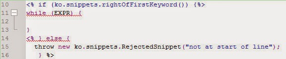
The script edit involves a few items below: Distinguish code properties by fonts, automatic syntax verification, code block collapse, code block indentation hint, auto-completion, function help, and computing result printout. In the following sections, we will write the scripts of the same function to compare the script edit function of these three types of IDE.

Since the detailed script algorithm is not important, we simply outline it, as shown below: Please make statistics on the sales volume of each department based on the sales.txt and employee.txt. Of which, EmployeeID is the associated field/column between these two files, Department is in the employee.txt, and employeeSales is in the sales.txt.

Perl

1. Distinguish code properties by fonts. The keywords, variables, constants, and comments are respectively presented in different fonts, clear and understandable at one glance.

2. Automatic syntax verification. This is a powerful function and quite useful for beginners. For example, since the row 31 is not properly written, IDE marks it with wavy line automatically. Programmers can simply put mouse pointer on the wavy line to view the hint in details.

To view all syntax verification results, click the "Grammar verification status" label below. In the below section, a few lines of scripts are written with errors purposefully to test the results: 

3.  Collapsing code block: There is a collapse button near the left row number , which can be used to collapse the code block and make the overall structure more clear. For example, collapse all code blocks, and the result would be like this:

4. Code block indentation hint. There are 5 vertical dash lines from row 14 to row 27, which clearly indicates the standardized indentation position to remind the programmer of writing the code up to the standard.

5.  Auto-completion function: IDE will auto-complete the whole function structure when programmers typing in the function name and press Tab key. For example, write WHILE and press down Tab key. The below contents will appear:

6.  Function help:

Perl does not have the true function help though, several workaround can barely implement this function.

Method 1: Function description: Hold down CTRL and then move the pointer to function. The function description will appear without any return value, parameter description, or examples. For example:

Method 2: Google search. Select function and hold down Shift+F1. IDE will open the browser of the operating system, and search for this function with Google, as shown below:

Method 3: Local manual search. Programmers can open the local Help from the Help menu, and press Ctrl+F to enter the keyword. The result is as follows:

It is obvious that none of the tree methods is convenient enough.

7.  Print the computing result.

The formal computing result will usually be output to file or database. Programmers will verify the result in the IDE. In the Perl, the computing result can be printed to the output console: 

Python

1. Python also uses different fonts to distinguish code properties, which is as easy-to-use as Perl does.

2. Automatic syntax verification. Python also provides the automatic syntax verification with the same wavy line indication. By pressing CTRL + F1, we can view the hint contents, as shown below:

Unlike Perl, Python does not provide the tab for syntax verification status. However, on the right side, we can still view the error summary clearly. This is similar to Eclipse. For example, if writing two lines of erroneous scripts on purpose, two red short lines will appear on the right, as shown below:

As for the automatic syntax verification, each of Python and Perl has its own merit. In my opinions, Python is more intuitive and convenient.

3. Code block collapsing. Although Python allows for code block collapsing, it is invalid for the FOR statement, but valid for the FROM statement which requires the collapse to the least. This function of Python has little practical value and worse than that of Perl.

4. Code block indentation hint. This IDE does not provide the code block indentation hint, and it is not as convenient as Perl.

5.   Auto-completion function. As long as the first few letters are typed-in, the IDE will give the candidate words.

If adding a full stop behind the object, the members of object can be listed directly, as shown below:

As for the auto-completion function, Python is more convenient than Perl.

6. Function help: Python provide much more convenient function help than that of Perl.

Hold down CTRL and put the mouse pointer on the function. The help for this function will appear, as shown below:

7. Computing result output

Like Perl, Python also allows for printing the computing result to the console by scripting, as shown below:

As can be seen, the output syntax of Python is much simpler than that of Perl. But the result is presented in a less friendly way than that in Perl. The data would become messy if there are plenty. To convert the Python output formate to table or list, composing more complex script is required.

esProc

1. esProc also uses different fonts to distinguish code properties, which is as easy-to-use as Perl and Python does. However, in esProc, only the comments, constants, and expressions can be distinguished. The esProc expressions can not be further classified to function name and variable name. What a pity.
2.  Automatic syntax verification. esProc does not offer the automatic syntax verification, which is inferior to Perl and Python in this regard. For example, if we write a statement with error in B2 cell intentionally, no hint will appear in IDE, as shown below:

The hint only appears when executing:

3. Code block collapsing. This IDE provides the code block collapse function which is at the same level to Perl and more practical than Python. Since the original algorithm is rather simple, and there is too few codes in IDE, we are unable to see the collapse effect. So, let's change to a complex syntax to demonstrate it, as shown below:

On the row 4, there is a collapse mark . Once clicked, the FOR statement will collapse, as shown below:

4. Code block indentation hint. esProc puts its script in a grid, and the grid line can be regarded as the natural indentation mark. The code is clear and easy-to-read without having to spare extra effort to lay out or align. The work scope of esProc code can be indicated clearly with the grid indentation. That is more convenient and much easier to read than the bracket adopted in Perl, and more intuitive than the Tab in Python. The indentation error can basically be avoided. Take the multi-level indentation in the below figure for example:

For the FOR statement in the A8 cell, the work scope is the indented cells B8-D23. Since A24 is not indented, the cell holds the next statement which is parallel to the FOR statement. By the same principle, the work scope of the IF statement in the B11 cell is from C12 to D17.

In Python, indentation is also used to represent the work scope. But the manual indentation is error prone. Programmers may easily confuse it with the continuous spaces and Tab. In addition, the indentation of Python brings a side effect: In Python, multiple statements are not allowed to put in a same row, while this restriction does not exit in esProc.

5. Auto-completion function. esProc does not have the auto-completion function and is inconvenient than Python in this regard

6.  Function help. The function help of esProc is similar to Python, which is much more convenient than that of Perl. Take the join function in the A2 cell for example. Simply put the cursor at the function name, and press “Alt+down arrow“ to view the description, return value, parameter, and parameter options for the join function.

7. Print the computing result. It is most comfortable to print the computing result in esProc. esProc is the grid-style script. The code is written in the cell. By clicking the cell, you can view the execution result in this cell, as shown below:

As can be seen, programmers are not required to write the code purposefully when printing the computing result in esProc. The data will be presented in a form fit for data type, for example, 2 dimension table, multilevel list, and single value. In comparison of this function, esProc is more friendly than Perl and Python.

Findings:

1. Distinguish code properties by fonts. These three IDE support this function well. By comparison, esProc is a bit inferior to them. To implement the same function, esProc script is much simpler. So, there will not be many confusions in reading.

2. Automatic syntax verification. Both Perl and Python support this function, and Python is a bit stronger, while esProc does not support this function.

3.  Code block collapsing. These three IDE support this function well. By comparison, Perl and esProc is more practical than Python.

4. Code block indentation hint. esProc is more convenient and intuitive than Perl, while Python does not provide the indentation hint at all.

5. Auto-completion function. Python provides the full support, and Perl is relatively poorer, while esProc does not provide the auto-completion function.

6. Function help. esProc and Python provide the perfect support, while Perl need improving in this aspect.

7.Print the computing result. Regarding the support, esProc is the best, while Python and Perl are almost at the same level.

Analysis:

Perl is a tool of traditional code line with support for the basic functions. Although not good enough in the function help, auto-completion, and output, the coding is not affected much.

Python makes some innovations on the traditional code lines: Use Tab indention to indicate the work scope with the concise syntax and hidden pointer. So, the length of code line in Python is a bit shorter than that in Perl. Although Python is not good enough regarding the indented hint and printout, they have less impact on coding.

esProc is a new grid-style code that represents the work scope using the intuitive grid indentation. Owing to this, esProc syntax is more concise, the esProc code for implementing the same function is several times shorter than that of Python. esProc also provide the fairly dedicated support for data processing. The data types of esProc include the common 2 dimension table objects and the multilevel list (generic set). The esProc functions and syntax are designed for the massive data. The result is presented in a way adapting to the data type automatically. One thing worthy noticing is that there is still great room for esProc to improve in the auto syntax verification and automatic completion. The lack in these two aspects could presently bring a certain degree of troubles to the usability.

4.Debugging comparison

In the practical development procedure, the bug debugging is usually more time-consuming than coding. So, it is one of the most important functions of IDE, and the key points of the comparison.

Perl

1.Debug and control functions. Perl provides the debugging and control functions, such as run to break point, run to cursor, step into, and step out. For example, set the break point to the 14th row. The result is as follows:

2.Monitoring variable.
There are many methods for monitoring variables in the Perl. First: View directly in the code zone by placing the mouse pointer to a certain variable in the code zone. IDE will hint the value of this variable directly. Take the @empArray variable in the row 12 for example:

This method is relatively intuitive, but the variable value is not completely displayed, appearing somewhat meaningless in practical use. To view the complete variable value, we need to take the second method. View in the variable list.

The only advantage of this method is that users can have a full view of the variable value. In other aspects, this method are disadvantageous. Take the complicated operations for example. Variables must be expanded to view the value. The variable @empArray as an example must be expanded for three times. For another example, the data monitoring is so inconvenient that users can neither view the row data transversally nor the column data vertically. This is a far cry from the structured data and extremely unfriendly. Take the below figure for example:

There is still another disadvantage for this method. Too many useless temporary variables distract the programmers’ attention seriously. For another example, only 2 variables are really useful to the row 14: @sales and @empArray. But the variable list lists 9 variables under Locals, and 6 variables under Globals, in addition to the 13 variables under Special. As can be imaged, how serious the interferences from the temporary variables could be when the program runs to the row 57 and puts to an end. To minimize the interference, we need to take the third method: watch.

In the section below, we will add @sales and @empArray to the Watch zone, as presented below:

As can be seen, the Watch function remedies some drawbacks of variable list to ensure that key variables can be free from the interferences of temporary variables. If Perl can improve the syntax agility, then it is certain that number of the temporary variables can be reduced fundamentally.

3. Temporary expression parsing. In debugging, we are often required to resolve the temporary expression outside the code. For example, view the second record of the variable @empArray, or the second field of the second record. In the watch window, this function is implemented, as shown below:

Perl supports this function well.

Python

1. Debug and control function. Python also provides the complete debug and control function. Similarly, we set the break point at a similar function as that in Perl, the result is shown below:

2. Monitoring variable.

The variable monitoring method for Python is similar to that for Perl. Method 1: View directly in the code zone. Move the mouse pointer to the empArray variable to view the variable value, as shown below:

Similar to Perl, the complete variable value cannot be monitored with this method. However, on clicking on the variable value, the complete variable value will expand in the window, as shown below:

2 dimension table! This is the very desired variable monitoring style to meet our very requirement. As can be seen, in Python, the variable value is almost the same as the structured data in the database or txt file. Although the vertical column is poorly aligned and there is no column name, it is quite convenient to view transversally. Judging from this point, Python is more friendly than Perl, and more convenient than program debugging.

Then, check out the method 2: View in the variable list.

In Python, variable can be viewed by simply expanding it once, which is more convenient than that in Perl, as shown below:

As can be seen, the variable list of Python solves two defects of Perl: Operation is complex, and variable presentation is not friendly. However, there are also quite a few useless temporary variables in the variable list of Python, which is similar to Perl.

The method 3 can solve the variable interference. The watch function of Python is shown below:

3. Temporary expression parsing

Python provides the convenient temporary expression parsing. For example, view the second record of the variable @empArray, or the second field of the second record.

Python also offers good support in this respect. In addition, because the variable presentation of Python is friendlier than that of Perl. So, the practical using experience of Python will also be better.

esPro

1. Debugging and control function. esProc provides the functions such as run to break point, run to cursor, step-by-step, and other debugging. But there is no step-into and step-out available. Fortunately, the step into/out can be replaced with step-by-step and run-to-cursor. So, not great inconvenience would be incurred. In addition, esProc code is concise. Since most loop statements in esProc can be replaced with functions, seldom would step into/out be used.

In esProc, the break point is set on the cells. Once set, the cell will be in pink, and the statement to which the program reaches will be in blue. For example, the breakpoint can be set at the similar location as that in Perl, and then enter the debug mode, as shown below:

2.  Monitoring variable. The variable monitoring method of esProc is more friendly than that for Perl/Python. Method 1: View in the code zone directly. Click the cell in esProc to view the cell value on the right, and the cell name is just the temporary variable name. For example, click the cell B1 - the temporary variable of B1 equals to the empArray in Python and Perl.

The variable value will be displayed to the full, as can be seen here. They are auto-sized and rendered in the form of tables. Because it is a table, a typical table has a column name, with row and column being aligned automatically. So, viewing in esProc is much convenient than that in Python and Perl.

Method 2: View in the variable list. The variables like A1 and B1 are temporary variables, not requiring the definition to make the reference directly. But for the meaningful variable, a name can be defined. For example, the associated computing result in A1 is named as data. Take the below figure for example:

As can be seen, there is no unnecessary temporary variables on the variable list of esProc. Every variable on list is meaningful. So, no such case as messy Perl/Python variables affecting each other would happen in esProc. Simply click once to view the esProc variable. For operation, it is as convenient as Python and much stronger than that of Perl. The variable is displayed as 2 dimension table with column name, which is more convenient than Python.

Method 3: watch. Watch is mainly used to reduce the interference of temporary variables. Therefore, the watch window is not required. Judging from this point, although esProc offers few functions, it is more convenient than Perl and Python, because those functions that esProc reduced are just the vulnerability and patches of Perl and Python.

3. Temporary expression parsing. Similarly, esProc supports the temporary expression parsing in the debug mode. For example, to get the first record of B1, we can directly write the expression in B2, or click on the Calculate cell button on the tool bar. The result is shown below:

You can define a variable to display in the variable list. For example, to define the field Name of the first record as name1, just type the below contents in B6: =name1=B1(1).Name. The result is:

As can be seen, the temporary expression parsing of esProc has the similar features to Python, and ever more stronger than Perl. Because esProc can use the table to adapt to and render the computing result, the actual user experience of esProc is better than that of Python.

Findings:

Debugging and control function. Perl and Python provide more complete debugging function. esProc lacks the step in/out, but the actual experiences does not differ greatly.

Monitoring variable. esProc is obviously superior to Python, and Python is more convenient than Perl.

Temporary expression parsing. esProc and Python are at the same level. Both are easier-to-use than Perl. The practical user experience of esProc is better than that of Python.

Analysis:

The grid-style of esProc is very characteristic. Users are not required to define the temporary variables. By doing so, the use of variable name can be reduced dramatically. The variable list becomes clear and practical, and patches such as watch window becomes unnecessary. esProc supports the structured 2 dimension table object, especially fit for the massive data processing, and more convenient for the variable monitoring. esProc code is more concise and further refined, resulting in smaller coding and debugging workload. Plus, esProc provides a great many loop functions to replace most loop statements, making the complex control method like step in/out unnecessary.

Python is a tool of traditional line-style code. There is an improvement, but somewhat redundant still. So there are quite a few unnecessary temporary variables, requiring the watch window to filter out the key variables. The variable monitoring of Python is convenient, allowing for the direct variable value monitoring, and presenting the data in a structured 2 dimension table.

Perl offers the traditional line-style code. The temporary variable is as messy as that of Python. A great deal of time is wasted on coding and debugging. It is not convenient to view the Perl variable, the operation is complex, and the display is not friendly enough. In the respect of temporary expression parsing, there are still some obstacle for Perl to overcome.