esProc Helps with Computation in MongoDB – Subquery

MongoDB doesn’t support the complex subquery which can only be realized by retrieving the data out first and then performing further computation. The operation is the same complex even if Java or other programming languages are used to write the program. In view of this, we can consider using esProc to help MongoDB with the computation, the method of which will be illustrated in detail through an example.

In MongoDB, there are two docments: orders, which stores the orders data, and employee, which stores the employee data. They are as follows:

> db.orders.find();

{ "_id" : ObjectId("5434f88dd00ab5276493e270"), "ORDERID" : 1, "CLIENT" : "UJRNP

", "SELLERID" : 17, "AMOUNT" : 392, "ORDERDATE" : "2008/11/2 15:28" }

{ "_id" : ObjectId("5434f88dd00ab5276493e271"), "ORDERID" : 2, "CLIENT" : "SJCH"

, "SELLERID" : 6, "AMOUNT" : 4802, "ORDERDATE" : "2008/11/9 15:28" }

{ "_id" : ObjectId("5434f88dd00ab5276493e272"), "ORDERID" : 3, "CLIENT" : "UJRNP

", "SELLERID" : 16, "AMOUNT" : 13500, "ORDERDATE" : "2008/11/5 15:28" }

{ "_id" : ObjectId("5434f88dd00ab5276493e273"), "ORDERID" : 4, "CLIENT" : "PWQ",

 "SELLERID" : 9, "AMOUNT" : 26100, "ORDERDATE" : "2008/11/8 15:28" }

…

> db.employee.find();

{ "_id" : ObjectId("5437413513bdf2a4048f3480"), "EID" : 1, "NAME" : "Rebecca", "

SURNAME" : "Moore", "GENDER" : "F", "STATE" : "California", "BIRTHDAY" : "1974-1

1-20", "HIREDATE" : "2005-03-11", "DEPT" : "R&D", "SALARY" : 7000 }

{ "_id" : ObjectId("5437413513bdf2a4048f3481"), "EID" : 2, "NAME" : "Ashley", "S

URNAME" : "Wilson", "GENDER" : "F", "STATE" : "New York", "BIRTHDAY" : "1980-07-

19", "HIREDATE" : "2008-03-16", "DEPT" : "Finance", "SALARY" : 11000 }

{ "_id" : ObjectId("5437413513bdf2a4048f3482"), "EID" : 3, "NAME" : "Rachel", "S

URNAME" : "Johnson", "GENDER" : "F", "STATE" : "New Mexico", "BIRTHDAY" : "1970-

12-17", "HIREDATE" : "2010-12-01", "DEPT" : "Sales", "SALARY" : 9000 }

…

It is required to select the orders data in which SELLERID is the EID of records of employees where STATE is California in employee. This can be expressed in SQL like this:

Select * from orders where orders.sellerid in (select eid from employee where employee.state=’ California’)。

The data of orders cannot be loaded entirely because their size is big, while the data size of both employee and the final result are not big.

The esProc script used to help MongoDB realize this subquery is as follows:

A1: Connect to MongoDB. localhost:27017 is the IP and the port number. test is the database name, user name as well as the password.

A2: Use find function to fetch the data from MongoDB and create a cursor. orders is the collection, with a filtering condition being null and _id , the specified key, not being fetched. Here esProc uses the same parameter format in find function as that in find statement of MongoDB. As esProc’s cursor supports fetching and processing data in batches, the memory overflow caused by importing big data all at once can thus be avoided.

A3: Fetch the desired data from employee according to the condition that STATE is California.

A4: Sort the EID field of A3’s employee data.

A5: Select the desired data from orders according to the condition requiring that SELLERID must exist in the table sequence in A4. That is, the condition can be expressed as SELLERID in A4. The resulting data can be loaded all at once. But if the data are too big, they can be fetched in batches. To fetch the top 1,000 rows, for example, can be expressed as fetch(1000).

The result is as follows:

Note：esProc isn’t equipped with a Java driver included in MongoDB. So to access MongoDB using esProc, you must put MongoDB’s Java driver (a version of 2.12.2 or above is required for esProc, e.g. mongo-java-driver-2.12.2.jar) into [esProc installation directory]\common\jdbc beforehand.

The esProc script used to help MongoDB with the computation is easy to be integrated into the Java program. You just need to add another line of code - result A6 to output a result in the form of resultset to Java program. For the detailed code, please refer to esProc Tutorial. In the same way, MongoDB’s Java driver must be put into the classpath of a Java program before the latter accesses MongoDB by calling an esProc program.

esProc Helps with Computation in MongoDB– Query Indexes in an Array

MongoDB can find out elements of a built-in array according to their indexes, but cannot find the indexes through the values of the elements. For example, the elements of an array are names of people stored according to their rankings. In MongoDB, names can be found according to the rankings (indexes of the array), but the values of rankings cannot be determined through names. esProc can help MongoDB in realizing this operation. The following example will teach you how it works in detail.

b–a collection of MongoDB, stores a name and an array of friends. The names in the array of friends are stored in the order of rankings, as shown below:

>db.b.find({"name":"jim"})

{ "_id" : ObjectId("544f3bf8cdb02668db9ab229"), "name" : "jim", "friends" : [ "t

om", "jack", "luke", "rose", "james", "sam", "peter" ] }

In MongoDB, you can find names through specified rankings. For example, find out the name of the first ranking among Jim’s friends:

>db.b.find({"name":"jim"},{"friends":{"$slice":[0,1]}})

{ "_id" : ObjectId("544f3bf8cdb02668db9ab229"), "name" : "jim", "friends" : [ "t

om" ] }

But you cannot find outthe ranking of “luke”,one of Jim’s friends. To solve the problem, esProc has its own script: 

A1: Connect to the MongoDB database. The IP and port number is localhost:27017, the database name is test and both the user name and the password are test. If any other parameters are needed, write them in line with the format mongo://ip:port/db?arg=value&…

A2: Fetch data from the MongoDB database using find function to create a cursor.The collection isb. The filtering criterion is name=jim and the specified keys are name and friends. It can be seen that this find function is similar to the find function of MongoDB. By fetching and processing data in batches, the esProc cursor can avoid the memory overflow resulting from big data importing.

A3: Since the data are not big, fetch function will fetch them all at once.

A4: Find out the position of luke using pos function.

After the code is executed, the result is as follows:

Please note that esProc hasn’t the java driver of MongoDB. To access MongoDB with esProc, the latter (a driver of 2.12.2 version or above is required, i.e. mongo-java-driver-2.12.2.jar) should be put into the [esProc installation directory]\common\jdbc beforehand.

The script for computation in MongoDB with the assistance of esProc is easy to integrate with Java program. By adding another line of code – A5, which is result A4, the result in the form of resultset can be output to Java program. For detailed code, please refer to esProc Tutorial. In the same way, to access MongoDB by calling esProc code with Java program also requires putting the java driver of MongoDB into the classpath of Java program.

esProc Helps with Computation in MongoDB – Digital Comparison

MongoDB script has limited computational ability in realizing complicated operations, so it is difficult to solve problems of this kind using it alone. In many cases, you can only perform further computations after retrieving the desired data out. And there is no less difficulty in trying to realizing this kind of set operations with high-level programming languages like Java. In this case, you can use esProc to help with the computation in MongoDB. An example will be provided for explaining how esProc works.

There is a collection – test – in MongoDB, as shown below:

> db.test.find({},{"_id":0})

{ "value" : NumberLong(112937552) }

{ "value" : NumberLong(715634640) }

{ "value" : NumberLong(487229712) }

{ "value" : NumberLong(79198330) }

{ "value" : NumberLong(440998943) }

{ "value" : NumberLong(93148782) }

{ "value" : NumberLong(553008873) }

{ "value" : NumberLong(336369168) }

{ "value" : NumberLong(369669461) }

…

Specifically, test includes multiple values, each of which is a digital string. It is required that each digital string be compared with all the other digital strings and find the biggest same digit and the biggest different digit in each digital string. If the number 1 exists both in the first row and in the nth row, their same digit will be counted as one. If the number exists only in the first row, and there is no such a number in the nth row, you can count one different digit.

esProc code:

A1: Connect to MongoDB. Both IP and the port number is localhost:27017. The database name, user name and the password all are test.

A2: find function is used to fetch data from MongoDB and create a cursor. orders is the collection, the filtering condition is null and _id , the specified key, won’t be fetched. It can be seen that esProc uses the same parameter format in find function as that in find statement in MongoDB. esProc’s cursor supports fetching and processing data in batches, thereby avoiding the memory overflow caused by importing big data at once. As the data size is not big, fetch function is used to get the records altogether from the cursor.

A3: Add two new columns to A2 for storing the biggest same and different numbers. And, at the same time, convert values into strings.

A4: Perform loop on the collection in A3, the loop body covers an area of B4-D10.

B4: Get the value on the current loop.

C4: Use array@s to split the column value into a sequence consisting of single characters and remove the duplicate values.

B5: Perform an inner loop on the collection in A3. The loop body is C6-D10.

C5: If the loop position of the inner loop is the same as the current one in the outer loop, that is, they hold the same value, skip the current inner loop and move on to the next.

C6: Get the value on the current inner loop.

C7: Define two variables - same and diff – for storing the same numbers and different numbers respectively got through the current comparison. The initial value is defined as zero.

C8: loop function is used to examine one by one in the inner loop the numerical values of the sequence formed by splitting values in the outer loop. If a same value is caught, the value of same will increase by one; otherwise the value of diff will increase by one.

C9, C10: Compare same and diff with those in A4, and reassign the bigger values to the same and diff in A4.

The final result after the code is executed is as follows:

Note: esProc isn’t equipped with a Java driver included in MongoDB. So to access MongoDB using esProc, you must put MongoDB’s Java driver (a version of 2.12.2 or above is required for esProc, e.g. mongo-java-driver-2.12.2.jar) into [esProc installation directory]\common\jdbc beforehand.

The esProc script used to help MongoDB in the computation is easy to be integrated into the Java program. You just need to add another line of code – A11 – that is, result A3, for outputting a result in the form of resultset to Java program. For the detailed code, please refer to esProc Tutorial. In the same way, MongoDB’s Java driver must be put into the classpath of a Java program before the latter accesses MongoDB by calling an esProc program.

esProc Helps with Computation in MongoDB – Sorting in Local Language

MongoDB uses unicode, instead of the coding for a certain local language, to sort data in this language (i.e. Chinese). Together with esProc, MongoDB can realize sorting in local language conveniently (i.e. sort Chinese according to Chinese phonetic alphabet). The following will teach you the method in detail by taking Chinese as an example.

person - a collection in MongoDB - stores names and genders as follows:

> db.person.find()

{ "_id" : ObjectId("544e4e070f03ad39eb2bf498"), "name" : "宋江", "gender" : "男"}

{ "_id" : ObjectId("544e4e070f03ad39eb2bf499"), "name" : "李逵", "gender" : "男"}

{ "_id" : ObjectId("544e4e070f03ad39eb2bf49a"), "name" : "吴用", "gender" : "男"}

{ "_id" : ObjectId("544e4e070f03ad39eb2bf49b"), "name" : "晁盖", "gender" : "男"}

{ "_id" : ObjectId("544e4e070f03ad39eb2bf49c"), "name" : "公孙胜", "gender" : "男" }

{ "_id" : ObjectId("544e4e070f03ad39eb2bf49d"), "name" : "鲁智深", "gender" : "男" }

{ "_id" : ObjectId("544e4e070f03ad39eb2bf49e"), "name" : "武松", "gender" : "男"}

{ "_id" : ObjectId("544e4e070f03ad39eb2bf49f"), "name" : "阮小二", "gender" : "男" }

{ "_id" : ObjectId("544e4e070f03ad39eb2bf4a0"), "name" : "杨志", "gender" : "男"}

{ "_id" : ObjectId("544e4e070f03ad39eb2bf4a1"), "name" : "孙二娘", "gender" : "女" }

{ "_id" : ObjectId("544e4e070f03ad39eb2bf4a2"), "name" : "扈三娘", "gender" : "女" }

{ "_id" : ObjectId("544e4e080f03ad39eb2bf4a3"), "name" : "燕青", "gender" : "男"}

…

Sort the data using MongoDB’s sort function rather than the Chinese phonetic alphabet:

> db.person.find({},{"name":1,"gender":1,"_id":0}).sort({"name":1})

{ "name" : "公孙胜", "gender" : "男" }

{ "name" : "吴用", "gender" : "男" }

{ "name" : "孙二娘", "gender" : "女" }

{ "name" : "宋江", "gender" : "男" }

{ "name" : "扈三娘", "gender" : "女" }

{ "name" : "晁盖", "gender" : "男" }

{ "name" : "李逵", "gender" : "男" }

{ "name" : "杨志", "gender" : "男" }

{ "name" : "武松", "gender" : "男" }

{ "name" : "燕青", "gender" : "男" }

{ "name" : "阮小二", "gender" : "男" }

{ "name" : "鲁智深", "gender" : "男" }

…

The esProc script helping with MongoDB computation is as follows:

A1：Connect to the MongoDB database. The IP and port number is localhost:27017, the database name is test and both the user name and the password are test. If any other parameters are needed, write them in line with the format mongo://ip:port/db?arg=value&…

A2：Fetch data from the MongoDB database using find function to create a cursor. The collection is person. The filtering criterion is null and the specified keys are name and gender. It can be seen that this find function is similar to the find function of MongoDB. By fetching and processing data in batches, the esProc cursor can avoid the memory overflow caused by big data importing.

A3：Since the data here are small, fetch function will fetch them all at once.

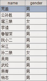
A4：Sort the data by name in ascending order, using sort function. Chinese is used in the data sorting. For the other localized languages esProc supports, please see below.

The result of operation is:

One thing to note is that esProc doesn't provide the java driver of MongoDB. To access MongoDB with esProc, the latter (a driver of 2.12.2 version or above is required, i.e. mongo-java-driver-2.12.2.jar) should be put into the [esProc installation directory]\common\jdbc beforehand.

The script for computation in MongoDB with the assistance of esProc is easy to integrate with Java program. By adding another line of code – A5, which is result A4, the result in the form of resultset can be output to Java program. For detailed code, please refer to esProc Tutorial. In the same way, to access MongoDB by calling esProc code with Java program also requires putting the java driver of MongoDB into the classpath of Java program.

The java driver of MongoDB can be downloaded from the following URL: https://github.com/mongodb/mongo-java-driver/releases.

esProc Simplifies SQL-style Computation – In-group Computation

During developing the database applications, we often need to perform computations on the grouped data in each group. For example, list the names of the students who have published papers in each of the past three years; make statistics of the employees who have taken part in all previous training; select the top three days when each client gets the highest scores in a golf game; and the like. To perform these computations, SQL needs multi-layered nests, which will make the code difficult to understand and maintain. By contrast, esProc is better at handling this kind of in-group computation, as well as easy to integrate with Java and the reporting tool. We’ll illustrate this through an example.

According to the database table SaleData, select the clients whose sales amount of each month in the year 2013 is always in the top 20. Part of the data of SalesData is as follows:

To complete the task, first select the sales data of the year of 2013, and then group the data by the month and, in each group, select the clients whose monthly sales amount is in the top 20. Finally, compute the intersection of these groups.

With esProc we can split this complicated problem into several steps and then get the final result. First, retrieve the data of 2013 from SaleData and group it by the month:

Note: The code for filtering in A2 can also be written in SQL.

It is the real grouping that esProc separates data into multiple groups. This is different from the case in SQL, whose group by command will compute the summary value of each group directly and won’t keep the intermediate results of the grouping. After grouping, the data in A3 are as follows:

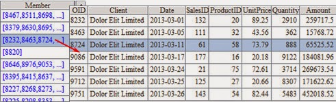
esProc will sorts the data automatically before grouping. Each group is a set of sales data. The data of March, for example, are as follows:

In order to compute every client‘s sales amount of each month, we need to group the data a second time by clients. In esProc, we just need to perform this step by looping the data of each month and group it respectively. A.(x) can be used to execute the loop on members of a certain group, with no necessity for loop code.

A4：=A3.(~group(Client))

In A4, the data of each month constitute a subgroup of each previous group after the second grouping:

At this point, the data of March are as follows:

It can be seen that each group of data in March contains the sales data of a certain client. 

Please note "~" in the above code represents each member of the group, and the code written with “~” is called in-group computation code, like the above-mentioned ~.group(Client).

Next, select the clients whose rankings of each month are in the top 20 through the in-group computation:

A5：=A4.(~.top(-sum(Amount);20))

A6：=A5.(~.new(Client,sum(Amount):MonthAmount))

A5 computes the top 20 clients of each month in sales amount by looping each month's data. A6 lists the clients and their sales amount every month. The result of A6 is as follows:

Finally, list the field Client of each subgroup and compute the intersection of the subgroups:

A7：=A6.(~.(Client))

A8：=A7.isect()

A7 computes the top 20 clients of each month in sales amount. A8 computes the intersection of the field Clients of the twelve months. The result is as follows:

As can be seen from this problem, esProc can easily realize the in-group computation, including the second group and sort, on the structured data, make the solving way more visually, and display a clear and smooth data processing in each step. Moreover, the operations, like looping members of a group or computing intersection, become easier in esProc, which will reduce the amount of code significantly.

The method with which a Java program calls esProc is similar to that with which it calls an ordinary database. The JDBC provided by esProc can be used to return a computed result of the form of ResultSet to Java main program. For more details, please refer to the related documents 

Features: esProc vs. SQL

Both can process mass structured data computing.

SQL is suitable for one-step-to-destination simple query. esProc is suitable for complex multi-step business logic.

esProc's advantages over SQL

Step computing, more thorough set operation, ordered computing, and object reference making computing much easier

Appropriate algorithm and data storage based on task features can gain better performance.

SQL's advantages over esProc

Universally applied, and many products with mature interface are available.

Transparent computing mechanism, regardless of data physical storage .

Related Topics:

The Disadvantages of SQL Computation (I)

The Disadvantages of SQL Computation (II)

The Disadvantages of SQL Computation (III)

Seven Drawbacks of Traditional OLAP

In 1993, E.F. Codd, the acknowledged founder of relational databases, introduced the term Online Analytical Processing (OLAP). OLAP is intended for the non-data processing professionals like the business expert, and is expected to be intuitive, rapid, and flexible.

  Intuitive user interface: clear a technical roadblock for business personnel to operate freely

  Rapid analysis procedure: accommodate the fast-changing business environment to seize opportunities and make decisions

  Flexible computing ability: able to confront many complex business computation

When the traditional OLAP product was just introduced, it experienced 2-digit growth rates in the global market for years before clients start to complain about that projects would easily fail, no obvious effect, and the time span is a bit too long. Since 2004, the growth of OLAP drops dramatically, owing to the seven major drawbacks of traditional OLAP tools(what’s the remedies of OLAP’s drawbacks?):

1. Pre-modeling as a must

Regarding the business data, the traditional OLAP tools do not allow for the immediate analysis without pre-modeling. These tools without a good OLAP engine cannot convert the data to a pattern in which business personnel can operate directly.

Assume that you are requested to analyze the profit for a telecommunications enterprise. Firstly, you need to draft a star or snowflakes model involving the date, region, client gender, client’s occupation, credit ratings, and other dimensions. Then, adapt the model to the practical database through repeated modifications. For example, remove the dimension of “customer’s occupation” from the model if it is not covered in the business data; replenish the ignored dimension of “hierarchy of consumption” to the analytical model; and use the ETL tool to synchronize the “sales network” from another database to this database. The finalized stable model will be filled with data regularly at scheduled times for use in analysis. Even so, you will find that the data is not up to the convention or short of historical data. Then, you will have to establish an additional data warehouse or data mart; In case no key data from the model is found, then you will return to modify the business system instead.

Modeling is a time-consuming procedure of a great many steps. Users thus have to pay the expensive cost in advance.

2. Great dependence on IT

Although business personnel is the intended user of OLAP, they will still have to work with the IT pros because the traditional OLAP tools requires a complex modeling procedure and its users have to write a great numbers of codes/scripts/SQL.

The below jobs cannot be completed without the assistance from technicians: Propose a common analytical model; Map dimensions of model to the names of fields, tables, and views of the business database; Use ETL tool or Perl scripts to migrate and integrate all required data to a same database if they are in different databases; Establish the reasonable scheduling rules, and fill data to the model by writing SQL statements or stored procedures; Deploy OLAP application to the server, and write .net/java application for user to use. Not to mention setting-up the database warehouse or data mart and modifying the business system to replenish the key data, business personnel is unable to handle without IT involvement.

The traditional OLAP tools depend heavily on the involvement of IT pros, and cost great human resources. What’s even worse, the IT pros without business expertise cannot fully understand the analysis goal. The model built by such IT pros may not be trustworthy enough. OLAP projects built through months or years of efforts often deviate away from the requirement of actual business, which gives rise to lots of project failures.

3. Poor computation capability

The data computing refers to a procedure of processing and transforming data through a series of specific steps toward a concrete goal. Data computing is a basic feature of OLAP. The traditional OLAP tools are of insufficient computational capabilities and few computational methods such as drilling, slicing, rotation, and simple column computation. This is because their architectures are old, lacking the innovation, and hard to strike a balance between user-friendliness and flexibility. Taking the below computational goal for example, it is hard to implement with the traditional OLAP tools.

How to find the workshop whose defective rate continuous to drop for 3 months in a row?

How to make statistics on students whose score on each course is above B?

In the 1st month since the new product enters the market, how many days will it takes to reach the 1/3 of the total sales in that month?

Lacking the computational capabilities impedes the flexibility of OLAP tool greatly. Analyzers are confined to a narrow and small area, incapable to analyze freely, and even have to resort to the 3rd party to perform this kind of computation. In the similar business computations, OLAP is often abandoned in an awkward situation.

4. Short of Interactive analysis ability

Data analysis is the most important feature of OLAP. Not like the data computing, data analysis is an interactive procedure requiring the perfect step-by-step computational mechanism. Toward the obscure goal, users need to observe the current data and make the reasonable assumption, and then verify/falsify the assumption to ultimately achieve the rather complicated business analysis goal. Unfortunately, the model of traditional OLAP tools is too old to provide so free a style of interactive analysis.

For example, why the sales improved greatly?

The possible assumptions include: orders flood in, sales forces beefed up in many respects, and any large orders are placed. Of which, the procedure to check the large orders is as given below:

1. List the order data, and then filter the data of recent 6 months.
2. Compute the average sales of each order.
3. Multiply the average sales by 300%, as the criterion of”large order” standard.
4. Group the data from step 2 by month, and filter the result from step 3 to get the large order.
5. View the result and lower the criterion for comparison if few orders are up to the criterion, and raise the criterion for comparison if there are too great orders after filtering.
6. Count the large orders of each month.
7. Compute the increment of large orders in each month.

Considering the above result, users may still need to keep investigating the cause of emerging large orders through computation until the clear and reliable basis for decision-making is found. The cause may be the vocational training for sales persons starts to bear fruit.

Traditional OLAP tools suffer from the limited interactive analysis abilities. They are unable to provide the above-mentioned flexible step-by-step computational capabilities, unable to solve the complex business computing, or provide the true basis for decision-making. So, quite a few clients just take OLAP tools as an expensive and apparently single-purpose reporting tool for presentation. They are trying to get more leverage, but only find the limited uses of OLAP for the time being.

5. Slow in reacting

Traditional OLAP tools require pre-molding and cooperation between people of various departments. Therefore, it is usually slow in reacting to the business analysis demands.

Assume that a toy manufacturer needs the below information before Christmas: Of the top 100 cities with the largest population, which cities require the sales effort being strengthened immediately. Then, you will find that no population data of the city in the existing model. The usage of traditional OLAP tools is as given below:

Business personnel download population data from census bureau or Wikipedia, and then use Excel and other similar tools to list the top 100 cities by population. The above step will not take more than 1 hour. But in the step followed, they will have to ask IT pros for help, because these data cannot be imported to OLAP for use directly.

Firstly, to coordinate: the business personnel raise a request to his/her superior. The superior will request the support from R&D department, and assign a project leader who will investigate the request initially, and build the project schedule and budget. The R&D department will approve and set up a development team. If cost is not a priority, then the development team can be standby all time for the business personnel.

Then, to implement: Perform the demand analysis in details and confirm it is to modify the model, schedule the task and export from Excel or database for other models to use. In addition, there are also steps of design, implementation, deployment, and verification as well as communication with database administers Web application administer, and programmers. When it comes to the final acceptance, further improvement is still required because IT pros may not be in the picture and are on the different page with business personnel. The improvement would be unavoidable unless unfortunately the Christmas was gone and they missed it.

The traditional OLAP is slow in reacting, requires great workload, and takes a bit too long time to implement the goal. Facing the fast-changing challenges, the enterprises will miss commercial opportunities, and find themselves in a disadvantage position in the intense competition.

6. Abstract model

The traditional OLAP tools convert the data of 2 dimensional from database and Excel to the multi-dimensional. To use the OLAP tools freely, business personnel must correctly understand the concepts of slicing, rotating, drilling, and other concepts as prerequisites. The abstraction of model hinders the business personnel from analyzing freely.

For example, to business personnel, the employee data, regional data, and product data are simply 3 lists or 3 sheets in Excel. Even the most ordinary business personnel know how to group, sort, and filter these data. However, things changes once these data is converted to the multi-dimensional data, business personnel have to say good bye to the data organized 2-dimensionally as flat as computer screen, and image these data as a cube. Never having the business personnel seen such data in their work or life before, they feel a bit tough to operate these abstract data.

The abstract model requires analyst to think 3-dimentionally. This gives rise to the difficulty to understand. Users are hard to convert the business language to the abstract multi-dimensional operations. Therefore, it is hard to truly implement the goal of on-line-analysis.

7. Great potential risk

Traditional OLAP tools have a huge potential risk due to the lacking of the computation and low interactive analysis ability, and the implementation relies on the cooperation with IT pros. The procedure and the cycle are a bit long.

The analyst are often forced to abandon the OLAP due to its poor computation ability that results in the failures to submit data of huge amount, and great difficulty to provide valuable references for the decision-maker. Lacking the interactive analysis ability, unable to solve the complex business analysis problem or find the true cause and solution, these drawbacks give rise to the faulty conclusion of analysis, and bring about great direct loss to the enterprise. In the analysis aimed to the business, too much work is relied on the IT pros. No wonder the procedure and cycle is lengthy, huge manpower and physical resources are consumed, while users are still unable to react effectively and efficiently to the constant changing business environment. Quite often, the ”stars” business is exceeded and ”cash cow” business is captured by others too. The analysis conclusion often deviates from the original goal of analysis, and the wrong decision may be easily made.

These potential risks can easily incur the failure of OLAP project, and bring about unrecoverable loss to the enterprise.

All in all, the traditional OLAP tools do not implement On Line Analytical Processing according to its true essence. They are just the “OLAP in its narrowest senses or the subset of OLAP”. It is neither intuitive nor fast or flexible.

Related Articles:

Script Computation of esProc Optimizes Analysts’ Benefits
Creative Spreadsheet Software for Data Processing in Development
Various Data Environments Support of esProc Makes Statistical Computing more Flexible