esProc Assists Report Development – Dynamic Datasources

Reporting tools, such as Jasper Report and BIRT, don’t have enough support for multi-datasources, leading to complicated Java program for realizing dynamic datasources. But by using esProc to assist the reporting tool, this won’t be a problem anymore. The following example will teach you how esProc works to realize the dynamic datasources.

myDB1 and myDB2 are different databases, but both have a table sales holding different data. We want to control the source of data of the report through the parameter PsCode and the range of data retrieval through the other two parameters – Pbegin andPend.

esProc code for doing this:

As you can see, esProc just uses a line of code to achieve using datasources dynamically.

sCode, begin and end are all esProc parameters. They can be set in the following window:  

begin and end are used to define the range of retrieving data from SQL and sCode is used to switch between datasources . The macro ${sCode} is to parse the parameters to get an esProc expression. To assign myDB2 to sCode, for instance, the above esProc script will be parsed into result myDB2.query("select * from sales where OrderDate>=? and OrderDate <=?",begin,end).

query function is used to execute an SQL statement, and receives parameters passed to it.

result statement will return the result to the reporting tool.

esProc provides JDBC interface to be integrated with the reporting tool, which will identify esProc as a database. For detailed integration solution, please refer to related documents

Next let’s take Jasper Report as an example to design a report. Its appearance and layout is as follows: 

Define three parameters – PsCode, Pbegin and Pend – in the report to correspond to the three esProc parameters. Click on Preview to see the completed report: 

In the above report, PsCode’s value is myDB1. We can change the value to myDB2 to see the effect of having dynamic datasources:  

Notice that the way a report calls the esProc script is the same as that it calls the stored procedure. If we save the script asdsource.dfx, then it can be called by dsource $P{PsCode},$P{Pbegin},$P{Pend} in Jasper Report’s SQL designer.

That the datasource name is directly used as the parameter, as in the first esProc script, may cause security problem. Sometimes users prefer to use numbers to represent the datasources. For instance, if PsCode’s value is 1, then retrieve data from myDB1; if the parameter has anotehr value, retrieve data from myDB2. This can be realized with the following code: 

This esProc script uses connect and close function to connect to or close the database explicitly, which features a higher flexibility.

esProc Assists Report Development – JOINs across MongoDB and MySQL

It is difficult to handle operations involving heterogeneous or multiple datasources, such as joins across MongoDB and MySQL, using the reporting tool, like Jasper Report, alone. Indeed Jasper Report and BIRT have the virtual data source or the table join and other functions to deal with them, but the functions are only provided in commercial or higher versions – because it’s hard to be provided for free – and have limited ability. They don’t support subsequent structured data computing on the joined data as SQL does.

esProc has a powerful structured data computing engine, supports heterogeneous datasources and is easy to be integrated. It is useful in assisting the reporting tool to realize joins across MongoDB and MySQL conveniently. Learn how esProc operates through the following example.

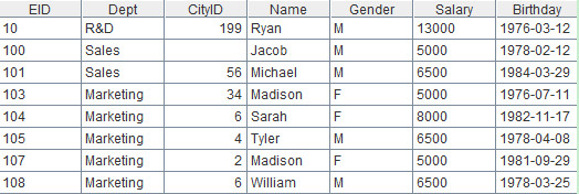
emp1 is a collection in MongoDB and cities is a table in MySQL. emp1’s CityID field, equivalent to a foreign key logically, points to cities’s CityID field. CityID and CityName are two fields of cities. What we want is to select employees from emp1according to a specified time interval and switch its CityID to CityName. Some of the source data are as follows:

Collection emp1

Table cities 

esProc script:

A1=MongoDB("mongo://localhost:27017/test?user=root&password=sa")

This line of code establishes the connection to MongoDB, in which user and password are parameters for specifying the user name and the password.

esProc supports to connect to MongoDB through JDBC as it does to connect to an ordinary database. But because the third-party JDBC is not as powerful as the official library function – for example, it cannot retrieve multilayer data, esProc encapsulates native methods directly, to retain MongoDB’s functions and syntax. Thus find function can be used.

A2=A1.find("emp1","{'$and':[{'Birthday':{'$gte':'"+string(begin)+"'}},{'Birthday':{'$lte':'"+string(end)+"'}}]}","{_id:0}").fetch()

This line of code retrieves records during a certain time interval from collection emp1 in MongoDB. find function’s first parameter is the collection name, its second parameter is the query condition that is defined according to syntax of MongoDB, and its third one is the specified field to be returned. Query condition’s two parameters- begin and end – are external parameters passed from the reporting tool, specifying respectively the beginning time and the ending time for Birthday.

find function returns a cursor. That means it won’t load all data into the memory at once and thus supports big data processing. The result cursor can be further processed by functions such as skip, sort, conj and etc. And data won’t be fetched until fetchfunction, groups function or for statement come into play. Suppose the time interval is from 1976-01-01 to 1988-12-31, then result of A2 is this:

A3=A1.close()

This line of code is used to close the connection to MongoDB established in A1.

A4=myDB1.query("select * from cities")

This line of code executes an SQL statement for retrieving data from MySQL, in which myDB1 is the datasource name. The configuration interface is as follows: 

It can be seen that the connection to the datasource is established through JDBC, which supports any database. In this way, the connection can be established and close either automatically or manually. Connection to MongoDB uses the latter way while this case adopts the former.

query function makes query through an SQL statement. Result is as follows: 

A5=A2.switch(CityID,A4)

This line of code replaces A2’s CityID field with A4’s corresponding records, with an effect similar to the left join. After the switching, A2 becomes like this (both A2 and A5 points to the same two-dimensional table): 

Click the blue hyperlink in CityID to see records in detail: 

Sometimes if an inner join is needed, use @i option in switch function. Then the code will be A2.switch@i(CityID,A4) and the result is as follows: 

A6=A5.new(EID,Dept,CityID.CityName:CityName,Name,Gender)

A5 establishes a relation between the collection and the table, while A6 retrieves from the result data the fields we want and creates a two-dimensional table using new function. CityID.CityName:CityName means retrieving CityName field corresponding to CityID field from A5 and renaming it CityName (for the reporting tool cannot identify field names like CityID.CityName).

As can be seen from the above code, after fields are switched by switch function, the database relation can be represented through object type access. This is simple and more intuitive, especially when establishing the multi-table and multilayer relation.

Result of A6 is as follows: 

That is all the data needed for creating the report. The final step is to return A6’s two-dimensional table to the reporting tool using result A6. esProc offers JDBC interface to be integrated with the reporting tool and the latter will identify it as a database. Learn more about the integration solution in related documents.

Then design the report with, for instance, JasperReport. The appearance and layout is as follows: 

Define two parameters – Pbegin and Pend – corresponding to the two esProc parameters in the report. Click Preview to see the report: 

esProc Assists Report Development – Computations Based on Multi-datasource Joins

Multiple datasources are very common in report development. We would first join tables from different databases before performing subsequent computations, such as filtering, grouping and sorting. With virtual data source or table join, reporting tools like JasperReport and BIRT can in some degree realize these computations based on joins between datasources. But they are difficult to master.

esProc, however, can be used to make the reporting tool’s handling of this situation easier, thanks to its powerful structured data computing, support for heterogeneous datasources and integration-friendly feature. The following is to illustrate how to deal with computations based on multiple datasources joins.

MySQL database has a table - sales - holding each day’s orders of more than one sellers and in which SellerId is the ID numbers of the sellers. emp is an MSSQL table having sellers’ information, in which EId is the ID numbers of the sellers, Name is their names and Dept is the departments. We want to display data of OrderID, OrderDate, Amount, Name and Dept in the report with the condition that order dates are limited to the past N days (say 30 days) or the data should belong to certain popular departments (like Marketing and Finance).

As orderID, OrderDate and Amount exist in sales while Name and Dept exist in emp, the two tables from different databases need to be joined first; then conditional filtering will be performed. Some of the source data are as follows:

Table sales

Table emp 

esProc code for doing this： 

A1=myDB1.query("select * from sales")

This line of code retrieves all records from sales of myDB1, which represents MySQL database. query function is used to execute SQL queries and can receive external parameters. A1’s result is as follows: 

A2=myDB2.query("select * from emp")

This line of code retrieves all records from emp of myDB2, which represents MSSQL database. 

A3=A1.switch(SellerId,A2:EId)

This line of code switches A1’s SellerId field to its corresponding records in A2 through the relational field EId. A3’s result is as follows (data items in blue have members of lower level): 

When there is no corresponding record for a data item in A1’s SellerId, switch function will by default retain the record this data item resides but display the record’s SellerId value as null. The effect is similar to the left join. If inner join is needed, use @ioption in the function, like A1.switch@i(SellerId,A2:EId).

        

A4=A3.select(OrderDate>=after(date(now()),days*-1)|| depts.array().pos(SellerId.Dept))

This line of code filters the result of join according to two conditions. The first one, represented by the expressionOrderDate>=after(date(now()),days*-1), is to select orders during the past N days (corresponding parameter is days); the second, represented by expression depts.array().pos(SellerId.Dept), is that the orders should belong to certain specified departments (corresponding parameter is depts). The operator “||” means the logical relationship “OR”.

now function represents the current time and date function converts it into the date. after function can represent the relative time, after("2015-01-30",-30), for example, means pushing the current time back by thirty days, i.e. 2015-01-01. With different options, the function can represent the relative time based on year, quarter, month and second.

array function converts a string into a set by the delimiter. "Marketing,Finance".array(), for instance, is equivalent to ["Marketing ","Finance"]. The function’s default separator is the comma, but we can specify other separators for it. pos function locates a member in the set, ["Marketing ","Finance"].pos("Finance"), for instance, is equivalent to 2 – or true logically. If the member doesn’t exist in the set, then null will be returned - which means false logically.

Note that SellerId.Dept represents the Dept field of the corresponding record of SellerId field. It can be seen that, after fields are switched by switch function, the table relation can be represented through object style access, which is intuitive and simple, especially when establishing the multi-table and multilayer relation.

days and depts are parameters passed from the reporting tool. If they get assigned with 30 and "Marketing,Finance" respectively, A4’s result will be as follows: 

A5=A4.new(OrderID,OrderDate,Amount,SellerId.Name:Name,SellerId.Dept:Dept)

This line of code gets fields the report needs from A4. SellerId.Name

and SellerId.Dept represent respectively Name and Dept in emp. The operator “:” means renaming. A5’s result is as follows: 

Now all data are ready for the report. Finally we just need to return A5’s two-dimensional table to the reporting tool with result A5. esProc offers the JDBC interface to be integrated with the reporting tool that will identify it as a database. See related documents for the integration solution.

Design a simple report using JasperReport, for instance. Its appearance and layout are as follows: 

Define two parameters – pdays and pdepts – in the report, corresponding to the two parameters in the esProc script. Click Preview to view the report: 

The way the reporting tool calls the esProc script is the same as that it calls the stored procedure. Save this script asafterjoin1.dfx, for instance, and it can be called by afterJoin1 $P{pdays},$P{pdepts} in JasperRreport’s SQL designer.

With the assistance of esProc, the reporting tool can tackle more complicated computations based on multi-dasource joins. To find out, for example, the top three days when each seller’s sales amount increases the most rapidly after a certain date, and to display names, dates of the three days, amount and growth rate.

esProc script: 

A1=myDB1.query("select * from sales where OrderDate>=?",beginDate)

This line of code retrieves orders after a certain date from sales, in which beginDate is the parameter passed from the reporting tool, whose value let’s assume to be “2015-01-01”. Then A1’s result is as follows: 

A2=myDB2.query("select * from emp")

This line of code retrieves all records from emp as follows: 

A3=A1.switch(SellerId,A2:EId)

This line of code switches A1’s SellerId field to its corresponding records in A2. Result is as follows: 

A4=A3.group(SellerId)

This line of code groups orders by SellerId. In the following figure, the left part is A4’s result and the right part shows two orders in detail. 

A5=A4.(~.groups(OrderDate,SellerId;sum(Amount):subtotal))

This line of code groups each SellerId’s orders by OrderDate and SellerId and summarizes the amount of each group. That is, it computes the sales amount of per seller per day. The result is as follows: 

In this line of code, “A4.()” means computing A4’s members by loop. “~” in the parentheses represents a variable of members, i.e. the record of order corresponding to a certain SellerId. “~.groups()” means applying groups function to each member. groupsfunction groups data and summarizes them simply, while group function only groups data.

A6=A5.(~.derive((subtotal-subtotal[-1])/subtotal[-1]:rate))

This line of code computes daily growth rate of the sales amount of each seller. The result is as follows: 

In this line of code, derive function is used to append a new field – rate – to each group. The arithmetic is “(sales amount of the current day – sales amount of the previous day)/ sales amount of the previous day”. We can see that subtotal[-1] is used in esProc to represent the sales amount of the previous day. This makes the computing of relative position easier.

Note that, since there is not the “sales amount of the previous day” for the first record, its growth rate is Null.

A7=A6.(~.select(#!=1))

This line of code removes the first record of each group in A6 (because its growth rate is a meaningless Null). 

select function queries records we want. “#” is the loop number and thus “#!=1” means the number is not equivalent to 1. The same effect can be achieved by delete function too, but with lower performance. That’s because the former returns only the references while the latter needs to modify the real data.

A8=A7.(~.top(-rate;3))

This line of code gets records of the top three days when the growth rate of each seller’s sales amount is the biggest. topfunction gets the top N records according to a certain field (or the expression of certain fields). A8’s result is as follows: 

A9=A8.union()

This line of code unions every group of data in A8 together to create a new two-dimensional table, as shown below: 

A10=A9.new(SellerId.Name:Name,OrderDate,subtotal,rate)

This line of code gets fields as required. Then the final result is as follows: 

result A10

This line of code returns A10’s two-dimensional table to the reporting tool. See the first example for the report design, which will be omitted here.

esProc Assists Report Development – Crosstab In Which Row & Column Headers Are Intervals

It is difficult to deal with some unconventional statistical tasks using the reporting tool, like Jasper and BIRT, alone or SQL. One example is the crosstab in which both the row headers and column headers are intervals, and whose measurement comes from anther database table. With powerful structured data computing engine and being integration-friendly, esProc can conveniently handle the case. I’ll explain the process of realizing dynamic data source through the following example.

account_no is the primary key of table account_detail, which has a one-to-many relationship with both table Paysoft_result andNAEDO through foreign key custno and foreign key customer_code. Report design requires that, according to the external parameters, empirica_score field of table account_detail be divided into segments that are used as the row headers and thatmfin_score field also be divided into segments that are used as the column headers. The computation of measurement is to divide the number of records of table Paysoft_result to which the account_no, which is the intersection-point where row headers and column headers meet, corresponds by that of table mfin_score to which it corresponds.

The following figure shows relations between the database tables and between certain fields and the report:

esProc will perform the data preparation using the following code:

A1=myDB1.query("select * from account_detail order by empirica_score,mfin_score")

This line of code retrieves data from table account_detail. myDB1 is the data source name that points to the database. queryfunction executes the SQL query statement. A1’s result is as follows:

A2=myDB1.query("select * from paysoft_result")

B2=myDB1.query("select * from NAEDO")

Then retrieve data from paysoft_result and NAEDO respectively in A2 and B2 likewise. Results are shown separately as follows:

A3=rowList.array()

B3=colList.array()

These two lines of code convert the parameters passed from the report into esProc sequences. Parameter rowList represents the row headers, like “560,575,585,595,605,615,625,635,645,654,665”, which includes ten consecutive intervals; parametercolList represents the column headers, like “39, 66, 91, 116, 137, 155”, which includes five consecutive intervals. array function is used to convert a string separated by commas into a sequence. The converting results are as follows:

A4=A1.select(empirica_score>=A3(1) && mfin_score>=B3(1))

In this example certain data in the source table exceed the range of the specified interval. For instance, customer “No501”’sempirica_sore is 540, which is smaller than the lower limit of the interval – 560. This line of code will filter out the data that are smaller than the lower limit in order to increase performance and simplify the expression.

select function executes data query or data filtering. empirica_score is a field of A1, A3(1) represents the first member of A3, i.e. 560, the lower limit of the interval. The logical operator “&&” means “AND”. A4’s result is as follows:

A5=A4.group(A3.pselect(empirica_score<~[1]):row,

  B3.pselect(mfin_score<~[1]):col;

  ~:accounts,

  A2.select(accounts.(account_no).pselect(~==custno)):p,

  B2.select(accounts.(account_no).pselect(~==customer_code)):n

)       

This line of code groups table account_detail in A4 according to the intervals in A3 (rowList) and those in B3(colList) and find out each group’s corresponding records in A2(paysoft_result) and B2(NAEDO).

group function is used to group data according to multiple fields (or grouping criteria). The syntax is A.group(field1,field2…). It is also used to compute subtotals or perform subsequent computations based on each group of data. The syntax isA.group(field1,field2… ; subtotal1,subtotal2…) . Fields of the grouped data can be renamed with “:new name”. The result of the above grouping operation contains five fields, which are row, col, accounts, p, n respectively. A5’s result is as follows:

To compute the grouping criterion row: Group A4’s empirica_score field according to A3’s intervals using the codeA3.pselect(empirica_score<~[1]). pselect function finds the sequence numbers of the eligible members in A3. “~” represents the current member of A3, ~[-1] represents its previous member and ~[1] represents the next one. The current interval is(empirica_score>=~ && empirica_score<~[1]). As all values of account_no field are bigger than the lower limit of the interval, the expression can be simplified as empirica_score<~[1]. According to “560,575,585,595,605,615,625,635,645,654,665”, A1 can be divided into 10 intervals - 560-574,575-584,585-594,595-604,605-614,615-624,625-634,635-644,645-654,655-664 – whose sequence numbers are from 1 to 10 in order.

To compute the grouping criterion col: Similarly, group A4’s mfin_score field according to B3’s intervals with the codeB3.pselect(mfin_score<~[1]). According to “39,66,91,116,137,155”, A1 can be divided into 5 intervals - 39-65,66-90,91-115,116-136,137-154 – whose sequence numbers are from 1 to 5 respectively.

Summary field account directly gets each group of data. “~” represents members of the current group. Click on accountscolumn highlighted in blue and the detail data will be displayed. For example, as the following figure shows, “row=1,col=1” corresponds the two intervals “560-574 and 39-65”; “row=2,col=5” corresponds the two intervals “575-584 and 137-154”:

To compute the summary field p: Find out records corresponding to accounts from A2 using the code A2.select(accounts.(account_no).pselect(~==custno)). select function accesses A2’s data and selects the eligible data by the filtering criterion. In the case of “row=1,col=1” and “row=2,col=5”, the records corresponding to column p are shown separately as follows (the relationship between accounts and A2 is one-to-many):

To compute summary field n: Similarly, find out records corresponding to accounts from B2 using the code B2.select(accounts.
(account_no).pselect(~==customer_code)). In the case of “row=1,col=1” and “row=2,col=5”, the records corresponding to column n are shown separately as follows:

A6=A5.derive(p.count():pCount,n.count():nCount)

This line of code appends to A5 the new columns pCount and nCount for computing the number of records of p and n in each group. The result is as follows:

A7=A6.derive(pCount/nCount:rate)

This line of code appends column rate to A6. The arithmetic is dividing pCount by nCount. The result is as follows:

A8=A7.run(string(A3(row))+"-"+string(A3(row+1)-1):row,string(B3(col))+"-"+string(B3(col+1)-1):col)

This line of code converts the sequence numbers in row field and col field into the corresponding intervals. run function performs the same computation on every member of A6 (a member is a row, where, for instance, row=1 and col=1). stringfunction converts a number into a string. The expression “A3()” gets A3’s members by their sequence numbers, A3(1), for instance, is 560. A8’s result is as follows:

The result of A8 contains the three fields the report requires. Then we only need to combine them into a new two-dimensional table and return it to the reporting tool through JDBC interface. This job will be done in A9 with the code result A8.new(row,col,rate).

new function retrieves the specified columns (or computed columns) from A8 to create a two-dimensional table. The result of executing A8.new(row,col,rate) is as follows:

Note: esProc provides the operator parentheses to compute the expressions separated by commas in order and return the last expression’s value. With the parentheses, the code from  A4 to A7 can be encapsulated into a single line:

A4=A1.select(empirica_score>=A3(1) && mfin_score>=B3(1)).group(

         A3.pselect(empirica_score<~[1]):row,

         B3.pselect(mfin_score<~[1]):col;

         (accounts=~,A2.count(accounts.(account_no).pselect(~==custno)) /

       B2.count(accounts.(account_no).pselect(~==customer_code))):rate

)

The result is as follows:

A9 is the data set the reporting tool needs. Now let’s design a simple crosstab with JasperReport in the following template:

Three points should be noted: Don’t place the crosstab in the detail band; configure the property of Data Pre Sorted as true; define parameters corresponding to those in the esProc script in the report, such as pRowLlist and pColList. A preview of the report is as follows:

The reporting tool calls the esProc script in the same way as that in which it calls the stored procedure. Save the esProc script as, say unregul.dfx, to be called by unregul $P{pRowList},$P{pColList} in JasperReport’s SQL designer. See related documents for detailed integration solution.