esProc Helps Process Heterogeneous Data Sources in Java –Cross-Database Relating

JoinRowSet and FilteredRowSet provided by RowSet– Java’s class library for data computing – can perform cross-database related computing, but they have a lot of weaknesses. First, JoinRowSet only supports inner join, it doesn’t support outer join. Second, test shows that db2, mysql and hsql can work with JoinRowSet, yet the result set of join oracle11g to other databases is empty though no error reporting will appear. The fact is there were two users who perform cross-database join using oracle11g database even got the correct result. This suggests that JDBC produced by different database providers will probably affect the result obtained by using this method. Last, the code is complicated.

esProc has proved its ability in assisting Java to perform cross-database relating. It can work with various databases, such as oracle, db2, mysql, sqlserver, sybase and postgresql, to perform a variety of cross-database related computing, like inner join and outer join involving heterogeneous data. An example will teach you the way esProc works. Requirement: relate table sales in db2 to table employee in mysql through sale.sellerid and employee.eid, and then filter data in both sales and employee according to the criterion state=”California”. The way the code is written in this task applies to situations where other types of databases are involved.

The structure and data of table sales are as follows: 

The structure and data of table employee are as follows:

Implementation approach: Call esProc script using Java program, join the multiple databases together to realize the cross-database relating, perform filtering and return the result to Java in the form of ResultSet.

The code written in esProc is as follows:

A1: Connect to the data source db2 configured in advance.

A2: Connect to the data source mysql configured in advance. In fact oracle and other types of databases can be used too.

A3, A4: Retrieve table sequences: sales and employee, from db2 and mysql respectively. esProc’s Integration Development Environment (IDE) can display the retrieved data visually, as shown in the right part of the figure in the above.

A5: Relate sales to employee through sellerid=eid using esProc’s object reference mechanism.

A6: Filter the two table sequences according to state="California".

A7: Generate a new table sequence and get the desired fields.

A8,A9: Close the connection

A10: Return the result to the caller of esProc program.

This piece of program is called in Java using esProc JDBC to get the result. The code is as follows (save the above esProc program as test.dfx):

//create a connection using esProcjdbc

Class.forName("com.esproc.jdbc.InternalDriver");

con= DriverManager.getConnection("jdbc:esproc:local://");

// call esProc program (the stored procedure) in which test is the name of file dfx

com.esproc.jdbc.InternalCStatementst;

st =(com.esproc.jdbc.InternalCStatement)con.prepareCall("call test()");

// execute esProc stored procedure

st.execute();

// get the result set

ResultSet set = st.getResultSet();

esProc Helps with Computation in MongoDB – Cross Summarizing

It is difficult for MongoDB to realize the operation of cross summarizing. It is also quite complicated to realize it using high-level languages, like Java, after the desired data is retrieved out. In this case, you can consider using esProc to help MongoDB realize the operation. The following example will teach you how it works in detail.

A collection – student – is given in the following:

db.student.insert  ( {school:'school1', sname : 'Sean' , sub1: 4, sub2 :5 })

db.student.insert  ( {school:'school1', sname : 'chris' , sub1: 4, sub2 :3 })

db.student.insert  ( {school:'school1', sname : 'becky' , sub1: 5, sub2 :4 })

db.student.insert  ( {school:'school1', sname : 'sam' , sub1: 5, sub2 :4 })

db.student.insert  ( {school:'school2', sname : 'dustin' , sub1: 2, sub2 :2 })

db.student.insert  ( {school:'school2', sname : 'greg' , sub1: 3, sub2 :4 })

db.student.insert  ( {school:'school2', sname : 'peter' , sub1: 5, sub2 :1 })

db.student.insert  ( {school:'school2', sname : 'brad' , sub1: 2, sub2 :2 })

db.student.insert  ( {school:'school2', sname : 'liz' , sub1: 3, sub2 :null })

We are expected to produce a cross table as the one in the following, in which each row is a school and the first column holds students whose results of sub1 are a 5 and the second column holds those whose results of sub1 are a 4 and so forth.

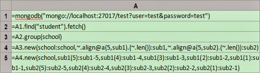
esProc script:

A1: Connect to MongoDB. Both IP and the port number are localhost:27017. The database name, user name and the password all are test.

A2: Use find function to fetch the collection – student - from MongoDB and create a cursor. Here esProc uses the same parameter format in find function as that in find statement of MongoDB. As esProc's cursor supports fetching and processing data in batches, the memory overflow caused by importing big data all at once can thus be avoided. In this case, the data can be fetched altogether using fetch function because the size is not big.

A3: Group the data by schools.

A4: Then group each group of data in alignment according to the sequence [1,2,3,4,5] and compute the length of each subgroup.

A5: Put the lengths got in A4 into corresponding positions as required and a record sequence wil be generated as the result.

The result is as follows:

Note：esProc isn't equipped with a Java driver included in MongoDB. So to access MongoDB using esProc, you must put MongoDB's Java driver (a version of 2.12.2 or above is required for esProc, e.g. mongo-java-driver-2.12.2.jar) into [esProc installation directory]\common\jdbc beforehand.

The esProc script used to help MongoDB with the computation is easy to be integrated into the Java program. You just need to add another line of code - result A6 to output a result in the form of resultset to Java program. For the detailed code, please refer to esProc Tutorial. In the same way, MongoDB's Java driver must be put into the classpath of a Java program before the latter accesses MongoDB by calling an esProc program.

Computing the Online Time for Users with esProc (IV)

In last article we mentioned that IT engineers from the Web Company used esProc to code single-machine multi-threaded program which could handle large data volume and complex requirements. This leverages the full power of one multi-core multi-CPU machine. Now once again these engineers found a new issue: with the user numbers for the online application growing explosively, colleagues from the Operation Department complained that the online time computation program is still running too slow.

IT Engineers leverage esProc's multi-machine parallel computing capability, to split the task for multiple machines to complete. The performance problem is resolved successfully. The single machine parallel processing is shifted to multi-machine parallel processing, with relatively low cost for hardware and software upgrade.

To improve performance, the Web Company increased the number of server from the original number of 1 to 3. Accordingly, the following steps are needed to shift from single-machine parallel to multi-machine parallel:

The first step: Modify the esProc program for weekly log files processing. Divide user ID by3 and separate the weekly log file into 3 files according to the remainder. Every server would be processing one of these. This way the file size were reduced and file transfer time could be shortened. Later the three files were uploaded to three servers, using multiple parallel programs to do the computation. The actual program is as following:

Note in the last screenshot that, A6 used the @g option of export function to retrieve "log files for one week" into three binary files. During subsequent use of parallel processing time, the content of log files can be retrieved by blocks for different user. The use of @g option is to ensure the segmented data retrieval is aligned to group borders, removing the possibility for assigning data of the same user to two blocks.

The second step: the single-machine multi-threaded program is unchanged. Let's go back.

Subroutine parameters are shown below. They are used to pass the log file name, block number and total number of blocks for the week when called by the main program. Here the log file name for the week, week file, was already one of the three segmented files corresponding to this machine.

The subroutine is as following:

The above screenshot illustrates that:

1. As we previously used export @g to output the file in group according to different user ID, the use of @z option by cursor in A2 to handle specific block (value is block number) among total (value is total blocks) from file will retrieve the complete group for the same userID. Data for one user will not be split into two blocks.

2.  The code line in red box returns the resulting file as cursor to the main program. Since multi-machine parallel processing were used here, this cursor is remote cursor ( Read esProc's Documents for detailed introduction on remote cursor).

The third step: writing main program for parallel computing, to call the parallel computing subroutine. As illustrated below, the main program called parallel tasks on tree machines, which effectively improved the performance for computation.

The server list in the program could also be written into the configuration file, this way any subsequent increase or decrease of the server would be easy.

Note: for specific measurements regarding esProc's performance gain with parallel computing, please refer to related test reports for esProc.Notes on the above screen capture:

1. callx@ parameter specifies 3 servers from A1 to A3, to handle three log files B1 to B3.

2. The syntax of callx's input parameter, is to specify three servers through A5, and specify 6 parallel computing tasks for each server in A6.

3. Server list, server number, and the number of tasks for each server can be adjusted according to actual situation, to leverage full performance potential of the server.

The fourth step: implement the esProc server, and upload related program & data files. Refer to instructions on esProc for specific steps and methods.

After the transformation to multi-machine parallel computing, the Operations Department found significant improvement in the computation speed of users online time. The cost of this transformation is much lower than that for application databases upgrade, especially, in the hardware part, only 2 additional PC Servers were needed.

So far, The Web Company finished implementation of esProc based user behavior analysis and computation platform. Its main advantages are:

1. The platform is easy to be adjusted with more complex algorithm for future, shortened the response time and saved labor costs from engineers.

2. It's easy to scale out for even larger data amount in the future, with shortened project time and reduced cost of upgrade.

Computing the Online Time for Users with esProc (III)

In last article we mentioned that IT engineers from the Web Company used esProc to code program which could handle large data volume and complex requirements. Not only could it meet the demands for online time computation, but also is relatively easy to be extended to with new conditions.

However, these engineers found that the single-threaded program does not take full advantage of the of the server's computing power. Practice has proved that the use of esProc's multi-threading capability can take advantage of the server's quaddual core, or even more CPUs. The change from single-threaded to multi-threaded requires very little workload. 

The Operation Department provided the following requirements for computation of users online time:
1. Login should be considered as the starting point of online time, and overnight should be take into consideration.

2. If the time interval between any two operations is less than 3 seconds, then this interval should not be added to online time.

3. If after login, the time interval between any two operations is longer than 600 seconds, then the user should be considered as logged out.

4. If there is only login, without logout, then the last operation time should be treated as time for logout.

5. For users who completed a post operation, his/her current time online time will be tripled in computation.

To shift from single-threaded computing to parallel computing, following steps needs to be done:

The first step: Adjust the log file preprocessor with the @g option of export function, to retrieve the log file for one week into a segmented binary file. In subsequent parallel processing, log file could be retrieved by block for different users. The use of @g option is to ensure the segmented data retrieval is aligned to group borders, removing the possibility for assigning data of the same user to two blocks. The actual procedures are as following:

The second step: Rewrite the online time computing program into a parallel subroutine. The part in the following red box is where we need to modify for parallel processing. Because different parallel tasks are used compute for different users, you can see that very little changes are required for parallel computing. The only change required, is to replace the use of files with different blocks from the binary file.

First we need to add parameters to subroutine, to pass the log file name, block number and total number of blocks for the week when called by the main program.

And then modify the program as following:

The above screenshot illustrates that:

1. As we previously used export@g to retrieve the file according to different user ID, the use of @z option by cursor to handle specific block (value is block number) among total (value is total blocks) from file, as shown in the redbox, will retrieve the complete group for the same userID. Data for one userwill not be split into two blocks.

2. A16 returns the resulting file as cursor to the main program.

The third step: writing main program for parallel computing, to call the parallel computing subroutine. Because the total cores of the server CPU is 8,the IT engineers decided to use six threads for parallel computing. This take full advantage of multi-core CPUs to improve performance.

Note: for specific measurements regarding esProc's performance gain with parallel computing, please refer to related test reports for esProc.

Upon the meeting of this requirement, IT engineers from the Web Company are facing a new problem: the user numbers for the online application grew explosively. Colleagues from the Operation Department complained that the online time computation program is still running too slow. The single-machine, multi-threaded approach can no longer enhance the computing speed significantly. Can these IT engineers effectively solve the performance issue using esProc’s parallel multi-machine computing capability? Is it too costly to transform to a multi-machine parallel mode? See "Computing the Online Time for Users with esProc (IV)"

Using esProc to Compute the Online Time of Users (I)

As the operator of an online system, the Web Company believes that the users' time spent with their online application is a key analysis scenario. Specifically, the online time refers to the cumulative time a user spent with their online business application over a certain period of time.

With the evolving of the company's online application, total number of users has grown and the task of user behavior analysis is becoming more complex. Here, we use the example of computing the online time for users to show the various computing scenarios, ranging from simple to complex. Hopefully this could serve as a reference for similar development projects. In fact, the following approach are also applicable for other categories of user behavior analysis, such as user's activity level, user churn, etc..

Let's start from the time when the application just went online. The Operation Department needed to know the user’s online time with their application every week. For this the engineers from IT department provided the following resolution.

The user behavior information is recorded in log files in the Web Company. Everyday a separatelog file is generated. For example, the following log file, "2014-01-07.log", contains the users online actions on January 7, 2014. To compute the online time for user in the week of 2014-01-05 to 2014-01-11, we need to retrieve data from 7 log files:

logtime    userid       action

2014-01-07 09:27:56        258872799       login

2014-01-07 09:27:57        264484116       login

2014-01-07 09:27:58        264484279       login

2014-01-07 09:27:58        264548231       login

2014-01-07 09:27:58        248900695       login

2014-01-07 09:28:00        263867071       login

2014-01-07 09:28:01        264548400       login

2014-01-07 09:28:02        264549535       login

2014-01-07 09:28:02        264483234       login

2014-01-07 09:28:03        264484643       login

2014-01-07 09:28:05        308343890       login

2014-01-07 09:28:08        1210636885     post

2014-01-07 09:28:09        263786154       login

2014-01-07 09:28:12        263340514       get

2014-01-07 09:28:13        312717032       login

2014-01-07 09:28:16        263210957       login

2014-01-07 09:28:19        116285288       login

2014-01-07 09:28:22        311560888       login

2014-01-07 09:28:25        652277973       login

2014-01-07 09:28:34        310100518       login

2014-01-07 09:28:38        1513040773     login

2014-01-07 09:28:41        1326724709     logout

2014-01-07 09:28:45        191382377       login

2014-01-07 09:28:46        241719423       login

2014-01-07 09:28:46        245054760       login

2014-01-07 09:28:46        1231483493     get

2014-01-07 09:28:48        266079580       get

2014-01-07 09:28:51        1081189909     post

2014-01-07 09:28:51        312718109       login

2014-01-07 09:29:00        1060091317     login

2014-01-07 09:29:02        1917203557     login

2014-01-07 09:29:16        271415361       login

2014-01-07 09:29:18        277849970       login

Log files record, in chronological order, users' operation (action), user ID (userid) and the time when the actions took place (logtime) in the application. Users operations include three different types, which are login, logout and get/post actions.

The Operation Department provided the following requirements for computation of users online time:
1. Login should be considered as the starting point of online time, and overnight should be take into consideration.

2. If the time interval between any two operations is less than 3 seconds, then this interval should not be added to online time.

3. If after login, the time interval between any two operations is longer than 600 seconds, then the user should be considered as logged out.

4. If there is only login, without logout, then the last operation time should be treated as time for logout.

As the online application was just rolled out, the data volume for log file is relatively small. To compute on data from log files for 2014-01-05 to 2014-01-11, we could retrieve all data into memory in one batch, or out to a resulting file. Thus all codes here are written for in-memory computing.

The IT Department leverages esProc to meet the above requirements.

The actualcodes are as following:


The ideas for program design are:

1. First, retrieve all log files for the week ( 2014-01-05 to 2014-01-11 ) and merge them in chronological order. Sorting them according to userid and logtime. Add two extra fields, online time and login flag for subsequent calculations.

2. Online time is for computing of the interval between two operations by the same user. If difference between the operation time of current line and last action is less than 3 seconds, or if the userid of current operation does not equal to that of last one, then online time is directly set to 0.

3. Login flag is used to indicate a valid online time. If onlinetime does not exceed 10 minutes (600 seconds), or the type of operation is logout, then loginflag is set to true. Otherwise it’s set to false. If it’s login operation, then login flag is directly set to true.

4. Upon the resulting sorted table from previous steps, compute login flag again.If loginflag was originally set to false,then leave it to false. If the value were originally set to true, then the type of last operation would result to different value. If the last operation were login, then login flag should still be set to true, otherwise it should be set to false.

5. Upon the resulting sorted table from previous steps, group the data according to userid. Compute the sum of onlinetime for all records whoseloginflag is true. This is the total online time for the same user.

6. Output the result in the last step to a file onlinetime.data.

The advantage of the above codes lies in the step-by-step way of computation, which is easy to maintain and modify.

After working for a while, a new problem was found: On the one hand, The Operation Department said that the original way for online time computation should be adjusted, with new conditions added. On the other hand, with the increase of users, the log files grow larger, which is too big to fit into memory in one batch. Well, how should the IT Departments cope with this change in the requirements? 

Please see "Computing the Online Time of users with esProc (II)".

Vector Computing Comparison: R Language vs. esProc

One of the most attractive features of R language and esProc is that their codes are both of the agile style, only requiring few lines of codes to implement plentiful functions. For example, both of them allow for composing Vector Computing expression, simplify the judgment statements, extend the basic functions to the advanced ones, and support the generic type. In which, regarding the vector computing, they are characterized with the massive data processing through functions and operators, so as to avoid the loop statement. Users can benefit from 2 resulting advantages: first, easy to grasp for developers and keep the learning cost low; second, easy to implement the computation and improve the performance.

Let’s compare the subtle differences between R and esProc on vector computing with several examples below.

Firstly, let’s check the most basic functions like vector value getting and assigning. For example, get 5 values of vectors whose subscripts are from 5 to 10, and replace them with another 5 values.

R:

01     A1<-c(51,52,53,54,55,56,57,58,59,60)

02     A2<-A1[6:10]

03     A1[6:10]<-seq(1,5)

esProc:

A1    =[51,52,53,54,55,56,57,58,59,60]

A2    =A1(to(6,10))

A3    >A1(to(6,10))=to(1,5)

Comments: Both of them enable users to get and assign values easily with almost the same usage. However, it seems that the “:” of R language to represent the interval ranges is very intuitive.

Then, let’s compare them on the arithmetical operations of vector.

R:

04     A4<-c(1,2,3)

05     A5<-c(2,4,6)

06     A4*A5      # multiplying the vector, and the result is: [1] 2 8 18

07     A4+2   #adding the vector to the constant, and the result is: [1] 345

08     ifelse(A4>1,A4+2,A4-2) 

              #conditional evaluate, and the result is: [1] -1  45

09     sum(A4)   #aggregate, sum up the vector member, and the result is:6

10     sort(A4,decreasing = TRUE)    #sort reversely, and the result is: 3 2 1

esProc:

A4       =[1,2,3]

A5       =[2,4,6]

A6       =A4**A5  ‘multiplying the vector, and the result is: 2 4 18

A7       =A4.(~+2)    

             ‘adding the vector to the constant, and the result is:3 4 5

A8       =A4.(if(~>1,~+2,~-2))       

             ‘conditional evaluate, and the result is:-1 4 5

A9       =A4.sum()     

             ‘aggregating, vector member sum up, and the result is:6

A10     =A4.sort(~:-1)  ‘reverse sorting, and the result is:3 2 1

Comments: As can be seen from the above, no matter the four arithmetic operations, aggregating, or sorting operations of vector, both R and esProc can implement it well, and their syntaxes are very close. One thing worthy of notice is that the code of esProc looks more “object-oriented”, while R is truly“object-oriented” judging from the bottom layer. The former is more suitable for direct use in common business sector, and the latter is more suitable for programmers to compile the extended package by themselves and more acceptable to those from the scientific expertise sector.

Let us check the vector computing on the structured data, such as computations based on the Orders table from the Northwind database:

1.Query the data with freightage from 200 to 300.

2.Query the order dated 1997.

3.Compute the intersection set of above-mentioned sets, i.e. data not only with freightage from 200 to 300 but also with orders placed in 1997.

4.Group the result from the previous step by EmployeeID, and average the freightage for each employee.

R:

02         A2<-result[result$Freight>=200 & result$Freight<=300,]

03         A3<- result[format(result$OrderDate,'%Y')=="1997",]

04         A4<-result[result$Freight>=200 & result$Freight<=300 & format(result$OrderDate,'%Y')=="1997",]

05         A5<-tapply(A2$Freight,INDEX=A2$EmployeeID,FUN=mean)

esProc :

A2         =A1.select(Freight>=200 && Freight<=300 && year(OrderDate)==1997)

A3         =A1.select(year(OrderDate)==1997)

A4         =A3^A4

A5         =A4.group(EmployeeID;~.avg(Freight))

Comments: R is good at querying and makes statistics in groups. However, as for the set operations, R is worse than esProc. In the above example of R, the result is obtained by an indirect means of query instead of any set operations.

R can only perform the set operations on simple vectors, for example, intersect(A2$Orderid,A3$Orderid), and cannot directly implement the set operation on the structured data like data.frame.

Of course, this is not to say that the R is not powerful in vector computing. In effect, R is easier to use than esProc in the aspect of matrix-related computation. For example, to seek the eigenvalue of matrix A, R users can simply use eigen(A), while esProc users are not provided with any functions for them to represent it directly.  Judging from this aspect, it proves that esProc is more suitable for business computing, while R is better in handling the scientific computation.

In conclusion, considering the vector computing, both R and esProc demonstrate perfect performance in the basic computing. More specifically speaking, R is second to none in matrix computation, and esProc is superior R in handling the structured data.